本文介绍了Hinton的第二篇胶囊网络论文“Matrix capsules with EM Routing”，其作者分别为Geoffrey E Hinton、Sara Sabour和Nicholas Frosst。我们首先讨论矩阵胶囊并应用EM（期望最大化）路由对不同角度的图像进行分类。对于那些想了解具体实现的读者，本文的第二部分是一个关于矩阵胶囊和EM路由的tensorflow实现。

CNN所面临的挑战

在上一篇关于胶囊的文章中，我们提到了CNN在探索空间关系中面临的挑战，并讨论了胶囊网络如何解决这些问题。让我们回顾一下CNN在分类相同类型但不同角度的图像时所面临的一些重要的挑战。例如，正确地分类不同的方向的人脸。

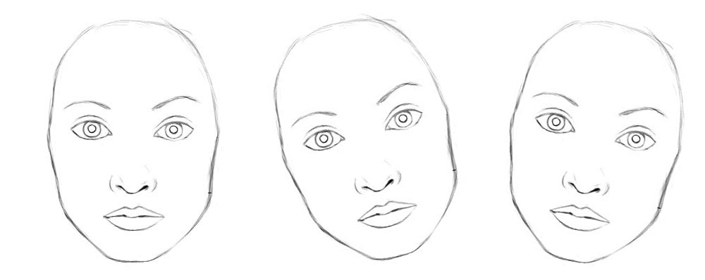
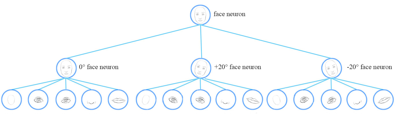
从概念上讲，CNN需要训练多个神经元来处理不同的特征方向（0°，20°，20°），并用一个顶层的人脸检测神经元检测人脸。

为了解决这个问题，我们添加了更多的卷积层和特征映射。然而，这种方法倾向于记住数据集，而不是概括解决方案。它需要大量的训练数据，去覆盖不同的变体以及避免过拟合。MNIST数据集包含55000个训练数据，每个数字有5500个样本。然而，小孩子们根本不需要这么多样本来学习数字识别。我们现有的深度学习模型，包括CNN，在利用数据上都显得非常低效。

对抗攻击

对于将个别特征进行简单的移动，旋转或大小调整的对抗样本，CNN显得非常脆弱。

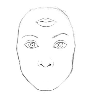
我们可以对图像添加微小的不可见的更改，从而轻松地欺骗一个深层神经网络。左边的图片被CNN正确地归类为熊猫。通过选择性地从中间图片向熊猫图片中添加微小的变化，CNN居然把右边的合成图像归类为长臂猿。

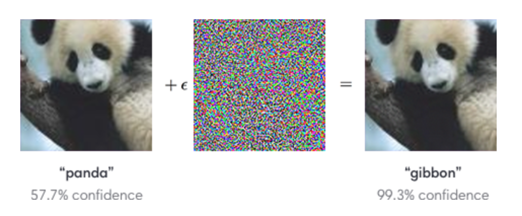
（图片来自 OpenAI）

胶囊

一个胶囊能够捕捉特征的可能性及其变体。因此，胶囊不仅能检测到特征，还能通过训练来学习和检测变体。

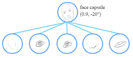
例如，同一网络层可以检测顺时针旋转的面部。

同变性是可以相互变换的对象的检测。直观地说，一个胶囊检测到脸右旋转20°（或左旋转20°），并不是通过匹配一个右旋转20°的变体来识别到脸部。通过迫使模型在胶囊中学习特征变量，我们可以用较少的训练数据更有效地推断可能的变体。在CNN中，最终的标签是视角不变的，即顶层神经元检测到一个人脸，但丢失了旋转角度信息。对于同变性来说，像旋转角度这类变化的信息被保存在胶囊里面。保留这些空间方向的信息可以帮助我们避免对抗样本攻击。

矩阵胶囊

一个矩阵胶囊同神经元一样可以捕捉激活（可能性），但也捕捉到了一个4x4的姿态矩阵。在计算机图形学中，一个姿态矩阵定义了一个物体的平移和旋转，它相当于一个物体的视角的变化。

(图片来源于论文Matrix capsules with EM routing)

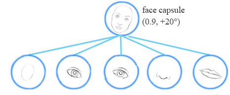
例如，下面的第二行图像代表上面同一对象的不同视角。在矩阵胶囊中，我们训练模型来捕捉姿态信息（方向、方位角等）。当然，就像其他深度学习方法一样，这仅仅是我们的意图，并不能得到保证。

(图片来源于论文Matrix capsules with EM routing)

EM（期望最大化）路由的目的是通过使用聚类技术（EM）将胶囊分组形成一个部分-整体关系。在机器学习中，我们使用EM聚类簇将数据点聚类为高斯分布。例如，我们通过两个高斯分布和建模，将下面的数据聚类为两簇。然后我们用对应的高斯分布来表示数据点。

在人脸检测这个示例中，低层中每一个嘴巴、眼睛和鼻子的检测胶囊都对其可能的父胶囊的姿态矩阵进行预测（投票）。每个投票都是父胶囊的姿态矩阵的一个预测值，它通过将自己的姿态矩阵乘以训练得到的 变换矩阵 WWW来计算。

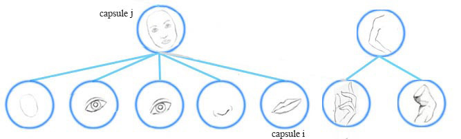
我们将在运行时使用EM路由，将胶囊分组到父胶囊中：

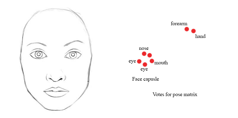
例如，如果鼻子，嘴和眼睛胶囊都有一个相似的姿态矩阵值的投票，那么我们将他们聚集在一起形成父胶囊：人脸胶囊。

A higher level feature (a face) is detected by looking for agreement between votes from the capsules one layer below. We use EM routing to cluster capsules that have close proximity of the corresponding votes.

高斯混合模型 & 期望最大化（EM）

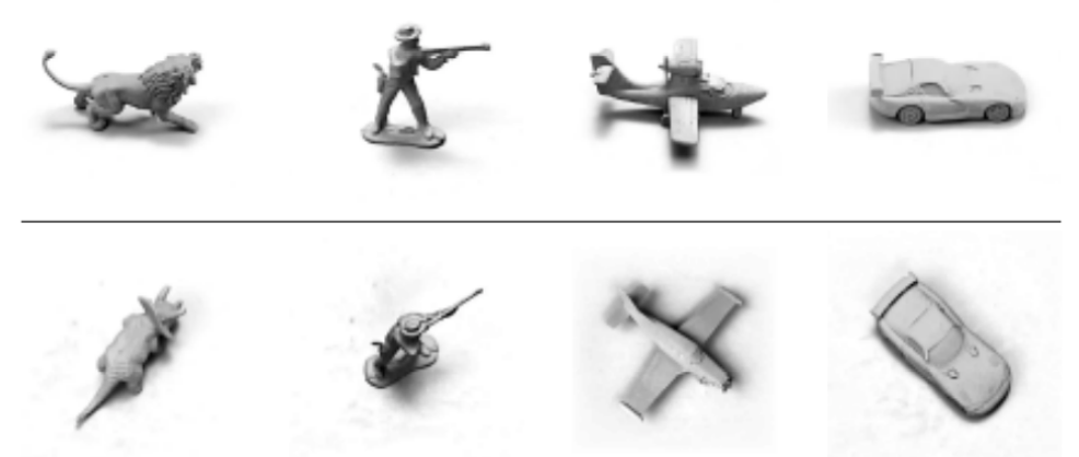
我们先来了解一下EM。高斯混合模型将数据点聚类为混合高斯分布，由均值μ" role="presentation" style="position: relative;">μμ\mu和标准差 σσ\sigma描述。下面，我们将数据点聚类为黄色和红色的集群，每一个都由不同的 μμ\mu和 σσ\sigma描述。

(图片来源于Wikipedia)

对于一个两集群的高斯混合模型，我们先随机的初始化集群和。期望最大（EM）算法通过将训练数据点拟合到G1G1G_1和G2G2G_2，然后基于高斯分布重新计算μμ\mu和σσ\sigma。将此过程不断迭代，直到解收敛，即在最终的G1G1G_1和G2G2G_2分布下，看到所有的数据点的概率最大化。

在给定集合G1G1G_1下，xxx的概率为：

在每次迭代中，我们开始于2个高斯分布，之后会根据数据点重新计算其μ" role="presentation" style="position: relative;">μμ\mu和σσ\sigma。

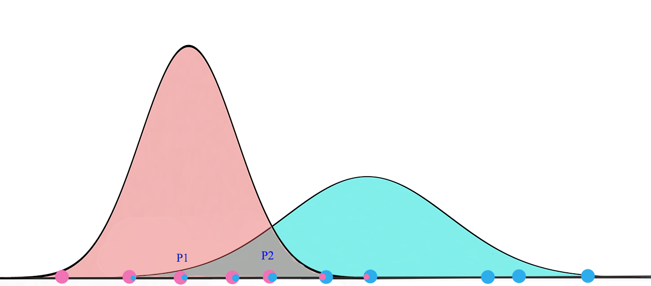
最终，我们会收敛到两个高斯分布，它使观察到的数据点的似然最大化。

使用EM进行协议路由（Routing-By-Agreement）

现在，我们探讨更多的细节。一个更高层次的特征（一张脸）通过寻找来自下一层胶囊的投票的协商被检测到。一个从胶囊iii到父胶囊j" role="presentation" style="position: relative;">jjj的投票vijvijv_{ij}可以通过将胶囊iii的姿态矩阵Mi" role="presentation" style="position: relative;">MiMiM_i乘以一个视角不变转换矩阵WijWijW_{ij}计算得到。

一个胶囊 iii作为一个部分-整体关系被归为胶囊j" role="presentation" style="position: relative;">jjj的概率是基于投票 vijvijv_{ij}与其他胶囊投票 (vo1j...vokj)(vo1j...vokj)(v_{o1j}...v_{okj})的接近程度。 WijWijW_{ij}通过成本函数和反向传播学到。它不仅学习了人脸的组成，而且能够保证在经过变换后父胶囊与其子组件的姿态信息匹配。

下面是矩阵胶囊的协议路由（Routing-By-Agreement）的可视化图。姿态矩阵TiTiT_i和TjTjT_j经视角不变矩阵转换后，根据投票的相似度，将胶囊分组。(TijTijT_{ij}与ThjThjT_{hj}即WijWijW_{ij}和WhjWhjW_{hj})

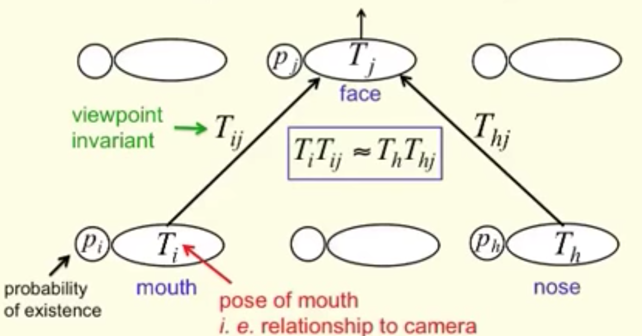
(图片来源于Geoffrey Hinton)

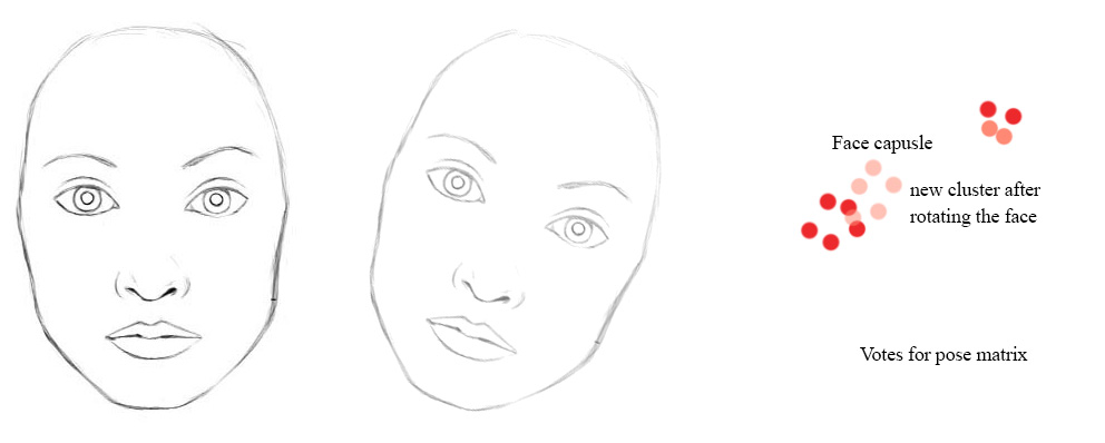
即使视角改变，姿态矩阵和投票也会以协调的方式变化。在我们的例子中，当脸部旋转时，选票的位置可能会从红色点变为粉红色点。然而，EM路由是基于邻近度的，它仍然可以将相同的子胶囊聚集在一起。因此，变换矩阵对于物体的任何视角都是相同的：视角不变性。用于对象的不同方向，我们只需要一组转换矩阵和一个父胶囊。

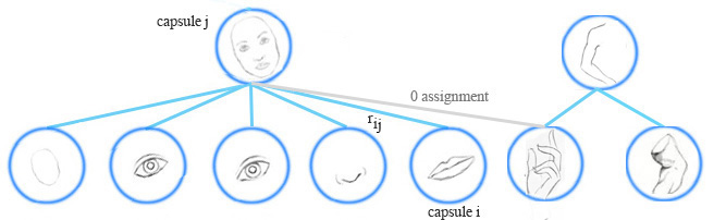
胶囊分配

EM路由在运行时将胶囊分组形成一个更高级别的胶囊。它同时会计算分配概率rijrijr_{ij}来量化胶囊及其父胶囊之间的运行时连接。例如，手胶囊不属于人脸胶囊，它们之间的分配概率为零。rijrijr_{ij}也被一个胶囊的激活程度所影响。如果图像中的嘴被阻塞，嘴胶囊将会有零激活值。计算出来的rijrijr_{ij}也将是零。

计算胶囊的激活值和姿态矩阵

胶囊输出的计算不同于深度网络的神经元。在EM聚类中，我们通过高斯分布来表示数据点。在EM路由中，我们仍用高斯模型对父胶囊的姿态矩阵进行建模。姿态矩阵是一个4×4矩阵，即16个元素。我们用具有16个μμ\mu和16个σσ\sigma的高斯模型对姿态矩阵建模，每个μμ\mu表示姿态矩阵的一个元素。

令vijvijv_{ij}为从胶囊iii到父胶囊j" role="presentation" style="position: relative;">jjj的投票，vhijvijhv_{ij}^h为它的第hhh个元素。我们应用高斯概率密度函数：

来计算vijh" role="presentation" style="position: relative;">vhijvijhv_{ij}^h属于胶囊jjj的高斯模型的概率：

取自然对数：

我们估算一下激活一个胶囊的成本。成本越低，胶囊就越有可能被激活。如果成本高，投票就不匹配父高斯分布，因此被激活的概率就越低。

令costij" role="presentation" style="position: relative;">costijcostijcost_{ij}为由胶囊iii激活父胶囊j" role="presentation" style="position: relative;">jjj的成本，它是对数似然取负：

由于低层的胶囊与胶囊 jjj有着不同的关联，我们根据运行时分配概率rij" role="presentation" style="position: relative;">rijrijr_{ij}按比例计算成本。所有下层胶囊的成本为：

我们用下面的公式来确定胶囊 jjj是否会被激活：

原文中，“−bij" role="presentation" style="position: relative;">−bij−bij-b_{ij}”被解释为描述胶囊 jjj的均值和方差的成本。换句话说，如果父胶囊j" role="presentation" style="position: relative;">jjj表示数据点的收益 bjbjb_j高于投票差异造成的成本，我们激活输出胶囊。我们不通过分析来计算 bjbjb_j。相反，我们通过反向传播和成本函数来训练它。

rijrijr_{ij}，μμ\mu，σσ\sigma和ajaja_j通过下一节讨论的EM路由迭代地计算。上述公式中的λλ\lambda是温度参数的倒数1temperature1temperature\frac{1}{temperature}。当rijrijr_{ij}越来越优，我们降低温度（λλ\lambda变大），它增加sigmoid(z)sigmoid(z)sigmoid(z)的S曲线的梯度。这有助于我们在这些区域内以更高的投票差异灵敏度更好地精调rijrijr_{ij}。在我们的实现里，迭代开始时λλ\lambda首先被初始化为1，然后每次路由迭代后增加1。论文并没有说明细节，我们建议在实现中采用不同的方案进行试验。

EM路由

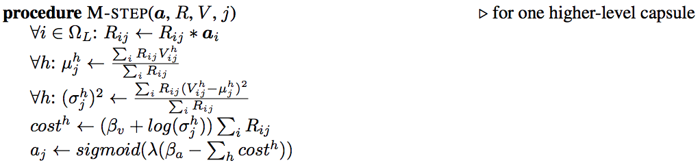
利用EM路由迭代计算出姿态矩阵和输出胶囊的激活值。EM法交替地调用步骤E和步骤M，将数据点拟合到混合高斯模型。步骤E确定父胶囊每个数据点分配的概率rijrijr_{ij}。步骤M在rijrijr_{ij}的基础上重新计算高斯模型的值。我们重复迭代3次。最终的ajaja_j就是父胶囊的输出。最终的高斯模型的16个μμ\mu将构成父胶囊的4×4姿态矩阵。

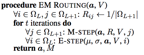
(图片来源于论文Matrix capsules with EM routing)

上面的aaa和V" role="presentation" style="position: relative;">VVV分别是激活值和子胶囊的投票。我们用均匀分布初始化分配概率rijrijr_{ij}。即开始时子胶囊与任意父胶囊有同样的关联。我们调用步骤M来计算更新的高斯模型(μ，σ)(μ，σ)(\mu，\sigma)和父激活ajaja_j，基于aaa，V" role="presentation" style="position: relative;">VVV和当前的rijrijr_{ij}。然后我们调用步骤E基于新的高斯模型和新的ajaja_j重新计算分配概率rijrijr_{ij}。

步骤M的细节：

在步骤M中，我们计算 μμ\mu和 σσ\sigma，基于子胶囊的激活 aiaia_i，当前 rijrijr_{ij}和投票 VVV。步骤M也会重新计算父胶囊的成本和激活aj" role="presentation" style="position: relative;">ajaja_j。 βvβv\beta_v和 βαβα\beta_\alpha会分别地训练。在我们的实现中，每一次路由迭代后 λλ\lambda（温度参数的倒数）增加1。

步骤E的细节：

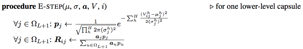
步骤E中，我们基于新的 μμ\mu， σσ\sigma和 ajaja_j重新计算分配概率 rijrijr_{ij}。如果投票越接近更新的高斯模型的 μμ\mu，分配则增加。

We use the ajaja_j from the last m-step call in the iterations as the activation of the output capsule jjj and we shape the 16 μ" role="presentation" style="position: relative;">μμ\mu to form the 4x4 pose matrix.

反向传播与EM路由的角色

在CNN中，我们用下面公式计算一个神经元的激活值：

然而，一个胶囊的输出，包括激活值和姿态矩阵，是通过EM路由计算得到的。我们使用EM路由计算父胶囊的输出，基于变换矩阵 WWW和子胶囊的激活值和姿态矩阵。然而，没有错误的情况下，矩阵胶囊仍然在很大程度上取决于通过反向传播训练的变换矩阵Wij" role="presentation" style="position: relative;">WijWijW_{ij}和参数 βvβv\beta_v和 βαβα\beta_\alpha。

在EM路由中，我们通过计算分配概率rijrijr_{ij}来量化子胶囊和父胶囊之间的连接。这个值很重要，但生命周期短暂。我们在EM路由计算前为每一个数据点使用均匀分布重新将它初始化。在任何情况，无论训练或测试，我们使用EM路由计算胶囊的输出。

损失函数（使用Spread损失）

矩阵胶囊需要一个损失函数来训练WWW，βv" role="presentation" style="position: relative;">βvβv\beta_v和βαβα\beta_\alpha。我们选择传播损失（spread loss）作为反向传播的主要损失函数。第iii类（不是真标签t" role="presentation" style="position: relative;">ttt）的损失被定义为：

atata_t是目标类（真标签）的激活值， aiaia_i是类 iii的激活值。

总损失为：

如果真标签和错误的类之间的边距小于m" role="presentation" style="position: relative;">mmm，我们通过 m−(at−ai)m−(at−ai)m-(a_t-a_i)的平方惩罚它。 mmm开始为0.2，在每一代训练后线性增加0.1。m" role="presentation" style="position: relative;">mmm达到最大值0.9后会停止增长。从较低的边距开始训练可以避免在早期阶段出现太多的死胶囊。

其他实现将正则损失和重构损失添加到损失函数中。由于这些对矩阵胶囊来说不重要，我们将在这里简单提到，不会进一步的阐述。

胶囊网络

在第一篇论文中胶囊网络（CapsNet）使用一个全连接网络。这个解决方案很难对较大的图像进行扩展。在接下来的几节中，矩阵胶囊使用CNN中的一些卷积技术来探索空间特征，以便能更好地扩展。

smallNORB

本论文的研究主要采用smallNORB数据集。它有5个玩具类：飞机、汽车、卡车、人和动物。每一个个体样本图有18种不同的方位角（0-340），9种高度和6种照明条件。该数据集特别适合于研究不同视角图像的分类。

(图片来源于论文Matrix capsules with EM routing)

架构

然而，许多代码实现始于MNIST数据集，因为其图像尺寸较小。所以我们的演示，同样挑选MNIST数据集。这是网络设计：

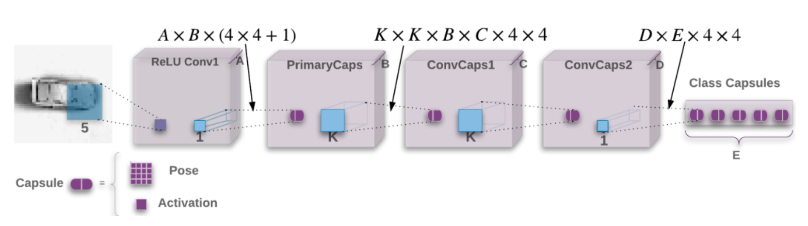
(图片来源于论文Matrix capsules with EM routing)

ReLU Conv1是一个常规的卷积层，其卷积核为5x5，步长为2，32（A=32）个输出通道（特征映射），激活函数为ReLU。

在PrimaryCaps层中，我们使用1x1的卷积核将32个通道转换为32（B=32）个初级胶囊，每个胶囊包含一个4x4矩阵和一个激活值。这里仍然使用常规的卷积层实现PrimaryCaps，并将每4x4+1个神经元组合为一个胶囊。

PrimaryCaps之后是一个**卷积胶囊层**ConvCaps1，卷积核为3x3（K=3），步长2。ConvCaps1使用胶囊作为输入和输出。ConvCaps1类似于常规的卷积层，不同的是，它使用EM路由来计算胶囊输出。

然后ConvCaps1的胶囊输出被喂给ConvCaps2。ConvCaps2是另一个卷积胶囊层，其步长为1.

ConvCaps2的输出胶囊通过1x1卷积核连接到Class Capsules，每一个分类由一个胶囊表示（在MNIST中，有10个类别，E=10）。

我们使用EM路由来计算ConvCaps1，ConvCaps2和Class Capsules的姿态矩阵和输出激活值。在CNN中，我们在空间维度上滑动相同的过滤器来计算同一特征映射。在检测相同的特征时不考虑位置。同样地，EM路由中，我们在空间维度上共享相同的转换矩阵WiWiW_i来计算投票。

例如，从ConvCaps1到ConvCaps2，我们有

一个3x3过滤器
32个输入、输出胶囊
一个4x4姿态矩阵

由于我们共享同样的转换矩阵，所以WWW仅需要3x3x32x32x4x4个参数

这里是每一层和其输出形状的汇总：

层	使用	输出形状
MNIST	图片	28, 28, 1
ReLU Conv1	常规卷积层，5x5卷积核，32个输出通道，步长为2，有填充	14, 14, 32
PrimaryCaps	改进的卷积层，1x1卷积核，步长为1，无填充，输出32个胶囊。共需要 32x32x(4x4+1)个参数。	pose (14, 14, 32, 4, 4), activations (14, 14, 32)
ConvCaps1	胶囊卷积，3x3卷积核，步长为2，无填充。共需要3x3x32x32x4x4个参数。	poses (6, 6, 32, 4, 4), activations (6, 6, 32)
ConvCaps2	胶囊卷积，3x3卷积核，步长1，无填充	poses (4, 4, 32, 4, 4), activations (4, 4, 32)
Class Capsules	胶囊卷积，1x1卷积核。共需要32x10x4x4个参数	poses (10, 4, 4), activations (10)

文章剩下的部分，我们将介绍一个基于Tensor的详细的实现。下面是构建这些网络层的代码：

def capsules_net(inputs, num_classes, iterations, batch_size, name='capsule_em'):"""Define the Capsule Network model"""with tf.variable_scope(name) as scope:# ReLU Conv1# Images shape (24, 28, 28, 1) -> conv 5x5 filters, 32 output channels, strides 2 with padding, ReLU# nets -> (?, 14, 14, 32)nets = conv2d(inputs,kernel=5, out_channels=32, stride=2, padding='SAME',activation_fn=tf.nn.relu, name='relu_conv1')# PrimaryCaps# (?, 14, 14, 32) -> capsule 1x1 filter, 32 output capsule, strides 1 without padding# nets -> (poses (?, 14, 14, 32, 4, 4), activations (?, 14, 14, 32))nets = primary_caps(nets,kernel_size=1, out_capsules=32, stride=1, padding='VALID',pose_shape=[4, 4], name='primary_caps')# ConvCaps1# (poses, activations) -> conv capsule, 3x3 kernels, strides 2, no padding# nets -> (poses (24, 6, 6, 32, 4, 4), activations (24, 6, 6, 32))nets = conv_capsule(nets, shape=[3, 3, 32, 32], strides=[1, 2, 2, 1], iterations=iterations,batch_size=batch_size, name='conv_caps1')# ConvCaps2# (poses, activations) -> conv capsule, 3x3 kernels, strides 1, no padding# nets -> (poses (24, 4, 4, 32, 4, 4), activations (24, 4, 4, 32))nets = conv_capsule(nets, shape=[3, 3, 32, 32], strides=[1, 1, 1, 1], iterations=iterations,batch_size=batch_size, name='conv_caps2')# Class capsules# (poses, activations) -> 1x1 convolution, 10 output capsules# nets -> (poses (24, 10, 4, 4), activations (24, 10))nets = class_capsules(nets, num_classes, iterations=iterations,batch_size=batch_size, name='class_capsules')# poses (24, 10, 4, 4), activations (24, 10)poses, activations = netsreturn poses, activations

ReLU Conv1

ReLU Conv1是一个简单的CNN层。我们使用Tensorflow slim API的slim.conv2d来创建CNN层，卷积核3x3，步长2，激活函数为ReLU。（使用slim API是为了使代码更精简，可读性更强）

def conv2d(inputs, kernel, out_channels, stride, padding, name, is_train=True, activation_fn=None):with slim.arg_scope([slim.conv2d], trainable=is_train):with tf.variable_scope(name) as scope:output = slim.conv2d(inputs,num_outputs=out_channels,kernel_size=[kernel, kernel], stride=stride, padding=padding,scope=scope, activation_fn=activation_fn)tf.logging.info(f"{name} output shape: {output.get_shape()}")return output

PrimaryCaps

PrimaryCaps层与CNN层没有太多的不同：它生成32个胶囊，其中每个胶囊包含一个4x4矩阵作为姿态矩阵，1个标量作为激活值，而不是像CNN一样仅生成一个标量。

def primary_caps(inputs, kernel_size, out_capsules, stride, padding, pose_shape, name):"""This constructs a primary capsule layer using regular convolution layer.:param inputs: shape (N, H, W, C) (?, 14, 14, 32):param kernel_size: Apply a filter of [kernel, kernel] [5x5]:param out_capsules: # of output capsule (32):param stride: 1, 2, or ... (1):param padding: padding: SAME or VALID.:param pose_shape: (4, 4):param name: scope name:return: (poses, activations), (poses (?, 14, 14, 32, 4, 4), activations (?, 14, 14, 32))"""with tf.variable_scope(name) as scope:# Generate the poses matrics for the 32 output capsulesposes = conv2d(inputs,kernel_size, out_capsules * pose_shape[0] * pose_shape[1], stride, padding=padding,name='pose_stacked')input_shape = inputs.get_shape()# Reshape 16 scalar values into a 4x4 matrixposes = tf.reshape(poses, shape=[-1, input_shape[-3], input_shape[-2], out_capsules, pose_shape[0], pose_shape[1]],name='poses')# Generate the activation for the 32 output capsulesactivations = conv2d(inputs,kernel_size,out_capsules,stride,padding=padding,activation_fn=tf.sigmoid,name='activation')tf.summary.histogram('activations', activations)# poses (?, 14, 14, 32, 4, 4), activations (?, 14, 14, 32)return poses, activations

ConvCaps1, ConvCaps2

ConvCaps1和ConvCaps2都是卷积胶囊层，其步长分别为2和1。在以下代码的注释中，我们会追踪ConvCaps1层的张量形状。

代码包括3个主要的部分：

使用kernel_tile来覆盖（卷积）之后投票和EM路由要用到的姿态矩阵和激活值
计算投票：调用mat_transform来生成投票，根据子胶囊中“tiled”的姿态矩阵和转换矩阵。
EM路由：调用matrix_capsules_em_routing来计算父胶囊的输出胶囊（姿态矩阵和激活值）。

def conv_capsule(inputs, shape, strides, iterations, batch_size, name):"""This constructs a convolution capsule layer from a primary or convolution capsule layer.i: input capsules (32)o: output capsules (32)batch size: 24spatial dimension: 14x14kernel: 3x3:param inputs: a primary or convolution capsule layer with poses and activationspose: (24, 14, 14, 32, 4, 4)activation: (24, 14, 14, 32):param shape: the shape of convolution operation kernel, [kh, kw, i, o] = (3, 3, 32, 32):param strides: often [1, 2, 2, 1] (stride 2), or [1, 1, 1, 1] (stride 1).:param iterations: number of iterations in EM routing. 3:param name: name.:return: (poses, activations)."""inputs_poses, inputs_activations = inputswith tf.variable_scope(name) as scope:stride = strides[1] # 2i_size = shape[-2] # 32o_size = shape[-1] # 32pose_size = inputs_poses.get_shape()[-1]  # 4# Tile the input capusles' pose matrices to the spatial dimension of the output capsules# Such that we can later multiple with the transformation matrices to generate the votes.inputs_poses = kernel_tile(inputs_poses, 3, stride)  # (?, 14, 14, 32, 4, 4) -> (?, 6, 6, 3x3=9, 32x16=512)# Tile the activations needed for the EM routinginputs_activations = kernel_tile(inputs_activations, 3, stride)  # (?, 14, 14, 32) -> (?, 6, 6, 9, 32)spatial_size = int(inputs_activations.get_shape()[1]) # 6# Reshape it for later operationsinputs_poses = tf.reshape(inputs_poses, shape=[-1, 3 * 3 * i_size, 16])  # (?, 9x32=288, 16)inputs_activations = tf.reshape(inputs_activations, shape=[-1, spatial_size, spatial_size, 3 * 3 * i_size]) # (?, 6, 6, 9x32=288)with tf.variable_scope('votes') as scope:# Generate the votes by multiply it with the transformation matricesvotes = mat_transform(inputs_poses, o_size, size=batch_size*spatial_size*spatial_size)  # (864, 288, 32, 16)# Reshape the vote for EM routingvotes_shape = votes.get_shape()votes = tf.reshape(votes, shape=[batch_size, spatial_size, spatial_size, votes_shape[-3], votes_shape[-2], votes_shape[-1]]) # (24, 6, 6, 288, 32, 16)tf.logging.info(f"{name} votes shape: {votes.get_shape()}")with tf.variable_scope('routing') as scope:# beta_v and beta_a one for each output capsule: (1, 1, 1, 32)beta_v = tf.get_variable(name='beta_v', shape=[1, 1, 1, o_size], dtype=tf.float32,initializer=initializers.xavier_initializer())beta_a = tf.get_variable(name='beta_a', shape=[1, 1, 1, o_size], dtype=tf.float32,initializer=initializers.xavier_initializer())# Use EM routing to compute the pose and activation# votes (24, 6, 6, 3x3x32=288, 32, 16), inputs_activations (?, 6, 6, 288)# poses (24, 6, 6, 32, 16), activation (24, 6, 6, 32)poses, activations = matrix_capsules_em_routing(votes, inputs_activations, beta_v, beta_a, iterations, name='em_routing')# Reshape it back to 4x4 pose matrixposes_shape = poses.get_shape()# (24, 6, 6, 32, 4, 4)poses = tf.reshape(poses, [poses_shape[0], poses_shape[1], poses_shape[2], poses_shape[3], pose_size, pose_size])tf.logging.info(f"{name} pose shape: {poses.get_shape()}")tf.logging.info(f"{name} activations shape: {activations.get_shape()}")return poses, activations

kernel_tile使用平铺和卷积来处理输入姿态矩阵和激活值，使其拥有正确的空间维度，为之后的投票和EM路由做准备（这段代码比较难懂，读者可将它看作一个黑盒）。

def kernel_tile(input, kernel, stride):"""This constructs a primary capsule layer using regular convolution layer.:param inputs: shape (?, 14, 14, 32, 4, 4):param kernel: 3:param stride: 2:return output: (50, 5, 5, 3x3=9, 136)"""# (?, 14, 14, 32x(16)=512)input_shape = input.get_shape()size = input_shape[4]*input_shape[5] if len(input_shape)>5 else 1input = tf.reshape(input, shape=[-1, input_shape[1], input_shape[2], input_shape[3]*size])input_shape = input.get_shape()tile_filter = np.zeros(shape=[kernel, kernel, input_shape[3],kernel * kernel], dtype=np.float32)for i in range(kernel):for j in range(kernel):tile_filter[i, j, :, i * kernel + j] = 1.0 # (3, 3, 512, 9)# (3, 3, 512, 9)tile_filter_op = tf.constant(tile_filter, dtype=tf.float32)# (?, 6, 6, 4608)output = tf.nn.depthwise_conv2d(input, tile_filter_op, strides=[1, stride, stride, 1], padding='VALID')output_shape = output.get_shape()output = tf.reshape(output, shape=[-1, output_shape[1], output_shape[2], input_shape[3], kernel * kernel])output = tf.transpose(output, perm=[0, 1, 2, 4, 3])# (?, 6, 6, 9, 512)return output

mat_transform提取转换矩阵参数作为一个可训练的Tensorflow变量w" role="presentation" style="position: relative;">www，然后将它与经过“tiled”处理的输入矩阵相乘，生成父胶囊的投票。

def mat_transform(input, output_cap_size, size):"""Compute the vote.:param inputs: shape (size, 288, 16):param output_cap_size: 32:return votes: (24, 5, 5, 3x3=9, 136)"""caps_num_i = int(input.get_shape()[1]) # 288output = tf.reshape(input, shape=[size, caps_num_i, 1, 4, 4]) # (size, 288, 1, 4, 4)w = slim.variable('w', shape=[1, caps_num_i, output_cap_size, 4, 4], dtype=tf.float32,initializer=tf.truncated_normal_initializer(mean=0.0, stddev=1.0)) # (1, 288, 32, 4, 4)w = tf.tile(w, [size, 1, 1, 1, 1])  # (24, 288, 32, 4, 4)output = tf.tile(output, [1, 1, output_cap_size, 1, 1]) # (size, 288, 32, 4, 4)votes = tf.matmul(output, w) # (24, 288, 32, 4, 4)votes = tf.reshape(votes, [size, caps_num_i, output_cap_size, 16]) # (size, 288, 32, 16)return votes

EM routing编码

这里是一个EM路由算法的实现，其交替地调用m_step和e_step。默认情况下，我们运行3次迭代。EM路由的主要目的就是计算输出胶囊的姿态矩阵和激活值。在最后一个迭代中，m_step已经完成了这些参数的最后估计。因此我们在最后一个迭代中跳过e_step，它对重新计算路由分配$r_{ij}起到了主要的作用。代码注释包含了ConvCaps1中张量形状的追踪。

def matrix_capsules_em_routing(votes, i_activations, beta_v, beta_a, iterations, name):"""The EM routing between input capsules (i) and output capsules (j).:param votes: (N, OH, OW, kh x kw x i, o, 4 x 4) = (24, 6, 6, 3x3*32=288, 32, 16):param i_activation: activation from Level L (24, 6, 6, 288):param beta_v: (1, 1, 1, 32):param beta_a: (1, 1, 1, 32):param iterations: number of iterations in EM routing, often 3.:param name: name.:return: (pose, activation) of output capsules."""votes_shape = votes.get_shape().as_list()with tf.variable_scope(name) as scope:# Match rr (routing assignment) shape, i_activations shape with votes shape for broadcasting in EM routing# rr: [3x3x32=288, 32, 1]# rr: routing matrix from each input capsule (i) to each output capsule (o)rr = tf.constant(1.0/votes_shape[-2], shape=votes_shape[-3:-1] + [1], dtype=tf.float32)# i_activations: expand_dims to (24, 6, 6, 288, 1, 1)i_activations = i_activations[..., tf.newaxis, tf.newaxis]# beta_v and beta_a: expand_dims to (1, 1, 1, 1, 32, 1]beta_v = beta_v[..., tf.newaxis, :, tf.newaxis]beta_a = beta_a[..., tf.newaxis, :, tf.newaxis]# inverse_temperature schedule (min, max)it_min = 1.0it_max = min(iterations, 3.0)for it in range(iterations):inverse_temperature = it_min + (it_max - it_min) * it / max(1.0, iterations - 1.0)o_mean, o_stdv, o_activations = m_step(rr, votes, i_activations, beta_v, beta_a, inverse_temperature=inverse_temperature)# We skip the e_step call in the last iteration because we only # need to return the a_j and the mean from the m_stp in the last iteration# to compute the output capsule activation and pose matrices  if it < iterations - 1:rr = e_step(o_mean, o_stdv, o_activations, votes)# pose: (N, OH, OW, o 4 x 4) via squeeze o_mean (24, 6, 6, 32, 16)poses = tf.squeeze(o_mean, axis=-3)# activation: (N, OH, OW, o) via squeeze o_activationis [24, 6, 6, 32]activations = tf.squeeze(o_activations, axis=[-3, -1])return poses, activations

等式中输出胶囊的激活值ajaja_j为

λλ\lambda是温度参数的倒数。在我们的实现中，开始为1，在每一个迭代中增加1。原论文并没有指定 λλ\lambda是如何增加的，你可以尝试不同的方案。这是我们的源码：

# inverse_temperature schedule (min, max)
it_min = 1.0
it_max = min(iterations, 3.0)
for it in range(iterations):inverse_temperature = it_min + (it_max - it_min) * it / max(1.0, iterations - 1.0)o_mean, o_stdv, o_activations = m_step(rr, votes, i_activations, beta_v, beta_a, inverse_temperature=inverse_temperature)

在最后一个迭代后，ajaja_j是最终的输出胶囊jjj的激活值。均值μjh" role="presentation" style="position: relative;">μhjμjh\mu^h_j用于相应姿态矩阵的第h个元素的最终值。我们稍后将这16个元素整理成一个4x4姿态矩阵。

# pose: (N, OH, OW, o 4 x 4) via squeeze o_mean (24, 6, 6, 32, 16)
poses = tf.squeeze(o_mean, axis=-3)# activation: (N, OH, OW, o) via squeeze o_activationis [24, 6, 6, 32]
activations = tf.squeeze(o_activations, axis=[-3, -1])

m-steps

m-steps的算法：

m_step计算父胶囊的均值和方差。ConvCaps1中均值和方差的形状分别为（24, 6, 6, 1, 32, 16）和（24, 6, 6, 1, 32, 1）。

以下是m-step方法的代码：

def m_step(rr, votes, i_activations, beta_v, beta_a, inverse_temperature):"""The M-Step in EM Routing from input capsules i to output capsule j.i: input capsules (32)o: output capsules (32)h: 4x4 = 16output spatial dimension: 6x6:param rr: routing assignments. shape = (kh x kw x i, o, 1) =(3x3x32, 32, 1) = (288, 32, 1):param votes. shape = (N, OH, OW, kh x kw x i, o, 4x4) = (24, 6, 6, 288, 32, 16):param i_activations: input capsule activation (at Level L). (N, OH, OW, kh x kw x i, 1, 1) = (24, 6, 6, 288, 1, 1)with dimensions expanded to match votes for broadcasting.:param beta_v: Trainable parameters in computing cost (1, 1, 1, 1, 32, 1):param beta_a: Trainable parameters in computing next level activation (1, 1, 1, 1, 32, 1):param inverse_temperature: lambda, increase over each iteration by the caller.:return: (o_mean, o_stdv, o_activation)"""rr_prime = rr * i_activations# rr_prime_sum: sum over all input capsule irr_prime_sum = tf.reduce_sum(rr_prime, axis=-3, keep_dims=True, name='rr_prime_sum')# o_mean: (24, 6, 6, 1, 32, 16)o_mean = tf.reduce_sum(rr_prime * votes, axis=-3, keep_dims=True) / rr_prime_sum# o_stdv: (24, 6, 6, 1, 32, 16)o_stdv = tf.sqrt(tf.reduce_sum(rr_prime * tf.square(votes - o_mean), axis=-3, keep_dims=True) / rr_prime_sum)# o_cost_h: (24, 6, 6, 1, 32, 16)o_cost_h = (beta_v + tf.log(o_stdv + epsilon)) * rr_prime_sum# o_cost: (24, 6, 6, 1, 32, 1)# o_activations_cost = (24, 6, 6, 1, 32, 1)# yg: This is done for numeric stability.# It is the relative variance between each channel determined which one should activate.o_cost = tf.reduce_sum(o_cost_h, axis=-1, keep_dims=True)o_cost_mean = tf.reduce_mean(o_cost, axis=-2, keep_dims=True)o_cost_stdv = tf.sqrt(tf.reduce_sum(tf.square(o_cost - o_cost_mean), axis=-2, keep_dims=True) / o_cost.get_shape().as_list()[-2])o_activations_cost = beta_a + (o_cost_mean - o_cost) / (o_cost_stdv + epsilon)# (24, 6, 6, 1, 32, 1)o_activations = tf.sigmoid(inverse_temperature * o_activations_cost)return o_mean, o_stdv, o_activations

E-steps

e-steps的算法：

e_step主要负责在m_step更新输出激活值 ajaja_j和高斯模型的 μμ\mu和 σσ\sigma后，重新计算路由分配（形状为：24,6,6,288,32,1）。

def e_step(o_mean, o_stdv, o_activations, votes):"""The E-Step in EM Routing.:param o_mean: (24, 6, 6, 1, 32, 16):param o_stdv: (24, 6, 6, 1, 32, 16):param o_activations: (24, 6, 6, 1, 32, 1):param votes: (24, 6, 6, 288, 32, 16):return: rr"""o_p_unit0 = - tf.reduce_sum(tf.square(votes - o_mean) / (2 * tf.square(o_stdv)), axis=-1, keep_dims=True)o_p_unit2 = - tf.reduce_sum(tf.log(o_stdv + epsilon), axis=-1, keep_dims=True)# o_p is the probability density of the h-th component of the vote from i to j# (24, 6, 6, 1, 32, 16)o_p = o_p_unit0 + o_p_unit2# rr: (24, 6, 6, 288, 32, 1)cdzz = tf.log(o_activations + epsilon) + o_prr = tf.nn.softmax(zz, dim=len(zz.get_shape().as_list())-2)return rr

Class capsules

回想前面几节，ConvCaps2的输出喂给Class capsules层。ConvCaps2的输出姿态矩阵形状为（24, 4, 4, 32, 4, 4）。

batch size为24
4x4空间输出
32个输出通道
4x4姿态矩阵

Class capsules使用1x1过滤器，而不是ConvCaps2中的3x3过滤器。它输出10个胶囊，每一个胶囊表示MNIST中10个类别中的一个，而不是一个2维的空间输出（ConvCaps1中为6x6，ConvCaps2中为4x4）。Class capsules的代码结构与conv_capsule相似。它调用方法计算投票，然后使用EM路由计算胶囊输出。

def class_capsules(inputs, num_classes, iterations, batch_size, name):""":param inputs: ((24, 4, 4, 32, 4, 4), (24, 4, 4, 32)):param num_classes: 10:param iterations: 3:param batch_size: 24:param name::return poses, activations: poses (24, 10, 4, 4), activation (24, 10)."""inputs_poses, inputs_activations = inputs # (24, 4, 4, 32, 4, 4), (24, 4, 4, 32)inputs_shape = inputs_poses.get_shape()spatial_size = int(inputs_shape[1])  # 4pose_size = int(inputs_shape[-1])    # 4i_size = int(inputs_shape[3])        # 32# inputs_poses (24*4*4=384, 32, 16)inputs_poses = tf.reshape(inputs_poses, shape=[batch_size*spatial_size*spatial_size, inputs_shape[-3], inputs_shape[-2]*inputs_shape[-2] ])with tf.variable_scope(name) as scope:with tf.variable_scope('votes') as scope:# inputs_poses (384, 32, 16)# votes: (384, 32, 10, 16)votes = mat_transform(inputs_poses, num_classes, size=batch_size*spatial_size*spatial_size)tf.logging.info(f"{name} votes shape: {votes.get_shape()}")# votes (24, 4, 4, 32, 10, 16)votes = tf.reshape(votes, shape=[batch_size, spatial_size, spatial_size, i_size, num_classes, pose_size*pose_size])# (24, 4, 4, 32, 10, 16)votes = coord_addition(votes, spatial_size, spatial_size)tf.logging.info(f"{name} votes shape with coord addition: {votes.get_shape()}")with tf.variable_scope('routing') as scope:# beta_v and beta_a one for each output capsule: (1, 10)beta_v = tf.get_variable(name='beta_v', shape=[1, num_classes], dtype=tf.float32,initializer=initializers.xavier_initializer())beta_a = tf.get_variable(name='beta_a', shape=[1, num_classes], dtype=tf.float32,initializer=initializers.xavier_initializer())# votes (24, 4, 4, 32, 10, 16) -> (24, 512, 10, 16)votes_shape = votes.get_shape()votes = tf.reshape(votes, shape=[batch_size, votes_shape[1] * votes_shape[2] * votes_shape[3], votes_shape[4], votes_shape[5]] )# inputs_activations (24, 4, 4, 32) -> (24, 512)inputs_activations = tf.reshape(inputs_activations, shape=[batch_size,votes_shape[1] * votes_shape[2] * votes_shape[3]])# votes (24, 512, 10, 16), inputs_activations (24, 512)# poses (24, 10, 16), activation (24, 10)poses, activations = matrix_capsules_em_routing(votes, inputs_activations, beta_v, beta_a, iterations, name='em_routing')# poses (24, 10, 16) -> (24, 10, 4, 4)poses = tf.reshape(poses, shape=[batch_size, num_classes, pose_size, pose_size] )# poses (24, 10, 4, 4), activation (24, 10)return poses, activations

为了整合class capsules中预测类的空间位置，我们为ConvCaps2中每个胶囊的投票的前两个元素的感受野中心添加缩放的x，y坐标。这称为Coordinate Addition。根据论文，这促进了模型训练变换矩阵，以生成这两个元素的值来表示特征相对于胶囊感受野中心的位置。Coordinate Addition的动机是利用投票的前2个元素(v1jk,v2jk)(vjk1,vjk2)(v^1_{jk},v^2_{jk})来推断预测类的空间坐标（x，y）。

通过保留胶囊中的空间信息，我们不再仅仅检查一个特性的存在。我们鼓励系统验证特征的空间关系，以避免对抗攻击。即如果特征的空间顺序错误，相应的投票就不匹配。

下面的伪代码说明了关键思想。ConvCaps2输出的姿态矩阵形状为（24, 4, 4,32, 4, 4）。即空间维度为4x4。我们使用的胶囊的坐标来定位在下面C1C1C1对应的元素（一个4x4矩阵），其含有空间胶囊的感受野中心缩放的x坐标。我们把这个元素的值增加v1ikvik1v^1_{ik}。对于投票的第二个元素v2jkvjk2v^2_{jk}，使用C2重复同样的过程。

# Spatial output of ConvCaps2 is 4x4
v1 = [[[8.],  [12.], [16.], [20.]],[[8.],  [12.], [16.], [20.]],[[8.],  [12.], [16.], [20.]],[[8.],  [12.], [16.], [20.]],]v2 = [[[8.],  [8.],  [8.],  [8]],[[12.], [12.], [12.], [12.]],[[16.], [16.], [16.], [16.]],[[20.], [20.], [20.], [20.]]]c1 = np.array(v1, dtype=np.float32) / 28.0
c2 = np.array(v2, dtype=np.float32) / 28.0

这里是最终的代码，看起来要复杂得多，以便处理任何大小的图像。

def coord_addition(votes, H, W):"""Coordinate addition.:param votes: (24, 4, 4, 32, 10, 16):param H, W: spaital height and width 4:return votes: (24, 4, 4, 32, 10, 16)"""coordinate_offset_hh = tf.reshape((tf.range(H, dtype=tf.float32) + 0.50) / H, [1, H, 1, 1, 1])coordinate_offset_h0 = tf.constant(0.0, shape=[1, H, 1, 1, 1], dtype=tf.float32)coordinate_offset_h = tf.stack([coordinate_offset_hh, coordinate_offset_h0] + [coordinate_offset_h0 for _ in range(14)], axis=-1)  # (1, 4, 1, 1, 1, 16)coordinate_offset_ww = tf.reshape((tf.range(W, dtype=tf.float32) + 0.50) / W, [1, 1, W, 1, 1])coordinate_offset_w0 = tf.constant(0.0, shape=[1, 1, W, 1, 1], dtype=tf.float32)coordinate_offset_w = tf.stack([coordinate_offset_w0, coordinate_offset_ww] + [coordinate_offset_w0 for _ in range(14)], axis=-1) # (1, 1, 4, 1, 1, 16)# (24, 4, 4, 32, 10, 16)votes = votes + coordinate_offset_h + coordinate_offset_wreturn votes

Spread loss

计算传播损失的等式：

mm<script type="math/tex" id="MathJax-Element-1855">m</script>的值从0.1开始。每一个迭代之后，我们将值增加0.1，直到达到0.9的最大值。这样可以防止在训练的早期阶段出现太多的死胶囊。

def spread_loss(labels, activations, iterations_per_epoch, global_step, name):"""Spread loss:param labels: (24, 10] in one-hot vector:param activations: [24, 10], activation for each class:param margin: increment from 0.2 to 0.9 during training:return: spread loss"""# Margin schedule# Margin increase from 0.2 to 0.9 by an increment of 0.1 for every epochmargin = tf.train.piecewise_constant(tf.cast(global_step, dtype=tf.int32),boundaries=[(iterations_per_epoch * x) for x in range(1, 8)],values=[x / 10.0 for x in range(2, 10)])activations_shape = activations.get_shape().as_list()with tf.variable_scope(name) as scope:# mask_t, mask_f Tensor (?, 10)mask_t = tf.equal(labels, 1)      # Mask for the true labelmask_i = tf.equal(labels, 0)      # Mask for the non-true label# Activation for the true label# activations_t (?, 1)activations_t = tf.reshape(tf.boolean_mask(activations, mask_t), shape=(tf.shape(activations)[0], 1))# Activation for the other classes# activations_i (?, 9)activations_i = tf.reshape(tf.boolean_mask(activations, mask_i), [tf.shape(activations)[0], activations_shape[1] - 1])l = tf.reduce_sum(tf.square(tf.maximum(0.0,margin - (activations_t - activations_i))))tf.losses.add_loss(l)return l

结论

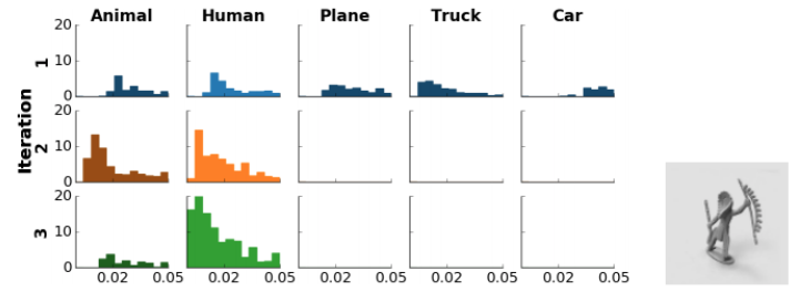
下面是每个路由迭代之后的5个最终胶囊的平均投票距离直方图。每个距离点由其分配概率加权。以人类图像作为输入，我们期望，经过3次迭代后，人类这一栏的差异最小（接近0）。（大于0.05的距离不在此显示）。

胶囊网络的错误率通常低于类似层数的CNN模型，如下所示。

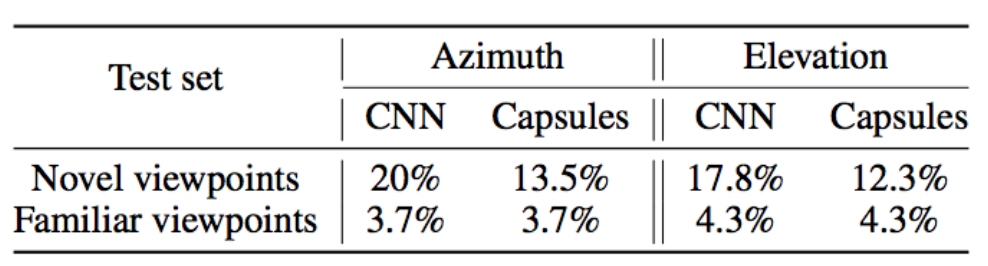
(图片来源于论文Matrix capsules with EM routing)

FGSM（快速梯度标志法）对抗样本的核心理念是在优化的每一步增加噪声，使分类从目标类偏移。它稍微修改图像，根据梯度信息最大限度地提高误差。相比CNN，矩阵路由不容易受到FGSM对抗样本的影响。

可视化

Class Capsules中的姿态矩阵被解释为图像的潜在表示。通过调节第一个2维姿态，并通过解码器重构（类似于之前的胶囊论文），我们可以将胶囊网络从MNIST数据中学到的信息可视化。

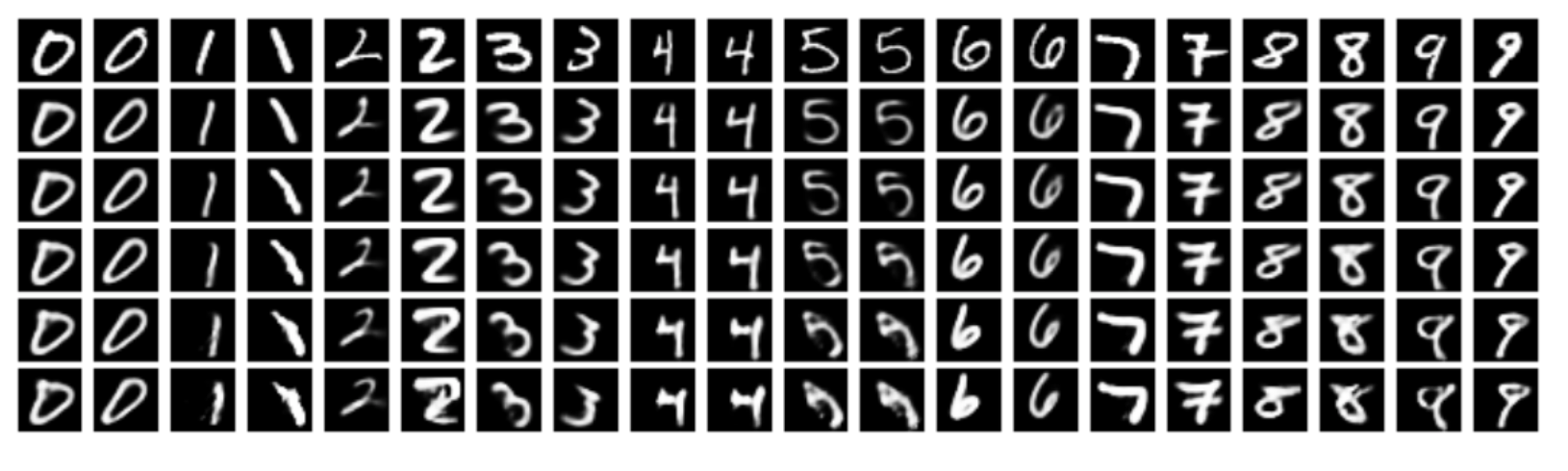
(图片来源于论文Matrix capsules with EM routing)

稍微旋转或移动一些数字，表明类胶囊学习到了MNIST数据集的姿态信息。

引用

计算投票和EM路由的部分代码是从Guang Yang和Suofei Zhang的实现修改而来。我们的源码放在github上，运行方式：

根据环境配置mnist_config.py和cap_config.py
运行train.py之前运行download_and_convert_mnist.py。

请注意，源代码只是为了演示目的，目前并没有支持。如果遇到问题，读者可参考其他实现。Zhang的实现似乎更容易理解，但Yang实现更接近原始文件。

原文链接：https://jhui.github.io/2017/11/14/Matrix-Capsules-with-EM-routing-Capsule-Network/

关于矩阵胶囊与EM路由的理解（基于Hinton的胶囊网络）相关推荐

第三十一课.矩阵胶囊与EM路由
矩阵胶囊的前向计算矩阵胶囊在向量胶囊的基础上改变了胶囊的表示方式,矩阵胶囊由激活概率与姿态矩阵两部分构成一个元组单位.激活概率用于表示矩阵胶囊被激活的概率,姿态矩阵用于表示胶囊的姿态信息.在向量胶囊 ...
三味Capsule：矩阵Capsule与EM路由
作者丨苏剑林单位丨广州火焰信息科技有限公司研究方向丨NLP,神经网络个人主页丨kexue.fm 事实上,在论文<Dynamic Routing Between Capsules>发布 ...
关于胶囊之间的动态路由的理解（基于Hinton的胶囊网络）
原文章:https://blog.csdn.net/bhneo/article/details/79391469 本文介绍了由Sara Sabour,Nicholas Frosst和Geoffrey ...
第三十课.向量胶囊与动态路由
向量胶囊的前向计算神经元用于检测一种确定的特征,而胶囊在检测特征的同时更注重描述这个特征.向量胶囊使用单位向量表达某种具体的特征,向量的模长反映该特征存在的概率.神经元与胶囊元的示意如图所示,(a) ...
ker矩阵是什么意思_如何理解正定矩阵和半正定矩阵
乍看正定和半正定会被吓得虎躯一震,因为名字取得不知所以,所以老是很排斥去理解这个东西是干嘛用的,下面根据自己和结合别人的观点解释一下什么是正定矩阵(positive definite, PD) 和半正 ...
【Umi+Dva入门实战】简述Dva、Umi和路由的理解
Umi 3+Dva入门实践–简述Dva.Umi和路由的理解 dva/umi/react 之间的关系 dva简介 umi简介 umi插件体系路由简介观看下面视频学习 https://www.bili ...
矩阵和数学空间的通俗理解，侵删
帮助初学者对矩阵和数学空间学习的理解和记忆注:转载自孟岩大佬的BLOG.链接发不出来就打了原创.侵删. 前不久chensh出于不可告人的目的,要充当老师,教别人线性代数.于是我被揪住就线性代数中一些 ...
【Web技术】913- 谈谈你对前端路由的理解
来自:掘金作者:尼克陈链接:https://juejin.cn/post/6917523941435113486 一篇文章,不可能做的面面俱到,全部受众.希望大家带着发散思维去看文章,将文章涉及的 ...
vue项目的一级路由和二级路由的理解
vue项目的一级路由和二级路由的理解

关于矩阵胶囊与EM路由的理解（基于Hinton的胶囊网络）

CNN所面临的挑战

对抗攻击

胶囊

矩阵胶囊

高斯混合模型 & 期望最大化（EM）

使用EM进行协议路由（Routing-By-Agreement）

胶囊分配

计算胶囊的激活值和姿态矩阵

EM路由

反向传播与EM路由的角色

损失函数（使用Spread损失）

胶囊网络

smallNORB

架构

ReLU Conv1

PrimaryCaps

ConvCaps1, ConvCaps2

EM routing编码

m-steps

E-steps

Class capsules

Spread loss

结论

可视化

引用

关于矩阵胶囊与EM路由的理解（基于Hinton的胶囊网络）相关推荐

最新文章

热门文章