This is series of how to developed data science project.

这是如何开发数据科学项目的系列。

This is part 1.

这是第1部分。

All the Life-cycle In A Data Science Projects-1. Data Analysis and visualization.2. Feature Engineering.3. Feature Selection.4. Model Building.5. Model Deployment.

数据科学项目中的所有生命周期-1 .数据分析和可视化2。 特征工程3。 功能选择4。 建立模型5。 模型部署。

This whole Data science project life cycle divided into 4 parts.

整个数据科学项目生命周期分为4个部分。

Part 1: How to analysis and visualize the data.

第1部分：如何分析和可视化数据。

Part 2: How to perform feature engineering on data.

第2部分：如何对数据执行特征工程。

Part 3: How to perform feature extraction.

第3部分：如何执行特征提取。

Part 4: model building and development.

第4部分：模型构建和开发。

This tutorial is helpful for them. who has always confused , how to developed data science projects and what is the process for developing data science projects.

本教程对他们有帮助。 谁总是困惑，如何开发数据科学项目以及开发数据科学项目的过程是什么。

So, if you are one of them . so you are at right place.

因此，如果您是其中之一。 所以你来对地方了。

Now, In this whole series. we gonna discuss about complete life cycle of data science projects. we will discuss from Scratch.

现在，在整个系列中。 我们将讨论数据科学项目的完整生命周期。 我们将从头开始进行讨论。

In this Part 1. we will see, how to analysis and visualize the data.

在第1部分中，我们将看到如何分析和可视化数据。

So, for all of this, we have to take simple data set of Titanic: Machine Learning from Disaster

因此，对于所有这些，我们必须采用“ 泰坦尼克号：灾难中的机器学习”的简单数据集

So, using this dataset we will see, how complete data science life cycle is work.

因此，使用该数据集，我们将看到完整的数据科学生命周期是如何工作的。

In next future tutorial we will take complex dataset.

在下一个未来的教程中，我们将采用复杂的数据集。

dataset link -https://www.kaggle.com/c/titanic/data

数据集链接 -https://www.kaggle.com/c/titanic/data

In this dataset 891 records with 11 features(columns).

在该数据集中，有11个特征(列)的891条记录。

So, let begin with part 1-Analysis and visualize the data in data science life cycle.

因此，让我们从第1部分开始分析，并可视化数据科学生命周期中的数据。

STEP 1-

第1步-

import pandas as pdimport numpy as npimport matplotlib as plt%matplotlib inline

Import pandas for perform manipulation on dataset.

导入熊猫以对数据集执行操作 。

Import numpy to deal with mathematical operations.

导入numpy以处理数学运算 。

Import matplotlib for visualize the dataset in form of graphs.

导入matplotlib在图表的形式直观的数据集。

STEP 2-

第2步-

data=pd.read_csv(‘path.csv’)data.head(5)

Dataset is like this-

数据集是这样的-

There is 11 features in dataset.

数据集中有11个要素。

1-PassengerId

1-PassengerId

2-Pclass

2类

3-Name

3名

4-Sex

4性别

5-Age

5岁

6-Sibsp

6麻痹

7-Parch

7月

8-Ticket

8票

9-Fare

9票价

10-cabin

10舱

11-embeded

11嵌入式

ABOUT THE DATA –

关于数据–

VariableDefinitionKeysurvivalSurvival0 = No, 1 = YespclassTicket class1 = 1st, 2 = 2nd, 3 = 3rdsexSexAgeAge in yearssibsp# of siblings / spouses aboard the Titanicparch# of parents / children aboard the TitanicticketTicket numberfarePassenger farecabinCabin numberembarkedPort of EmbarkationC = Cherbourg, Q = Queenstown, S = Southampton

VariableDefinitionKeysurvivalSurvival0 =否，1 = YespclassTicket class1 = 1st，2 = 2nd，3 = 3rdsexSexAgeAge年龄在Titanicparch的同胞/配偶中的同胞/配偶数＃TitanicticketTicket的票价/乘客乘母票的票价是南安普敦

可变音符 (Variable Notes)

pclass: A proxy for socio-economic status (SES)1st = Upper2nd = Middle3rd = Lower

pclass ：社会经济地位(SES)的代理人1st =上层2nd =中间3rd =下层

age: Age is fractional if less than 1. If the age is estimated, is it in the form of xx.5

age ：年龄小于1时是小数。如果估计了年龄，则以xx.5的形式出现

sibsp: The dataset defines family relations in this way…Sibling = brother, sister, stepbrother, stepsisterSpouse = husband, wife (mistresses and fiancés were ignored)

sibsp ：数据集通过这种方式定义家庭关系… 兄弟姐妹 =兄弟，姐妹，继兄弟，继母配偶 =丈夫，妻子(情妇和未婚夫被忽略)

parch: The dataset defines family relations in this way…Parent = mother, fatherChild = daughter, son, stepdaughter, stepsonSome children travelled only with a nanny, therefore parch=0 for them.

parch ：数据集通过这种方式定义家庭关系… 父母 =母亲，父亲孩子 =女儿，儿子，继女，继子有些孩子只带保姆旅行，因此parch = 0。

STEP 3 -After import the dataset. now time to analysis the data.

步骤3-导入数据集后。 现在该分析数据了。

First, we gonna go check the Null value in dataset.

首先，我们要检查数据集中的Null值。

null_count=data.isnull().sum()null_count

In that code-

在该代码中-

Now here, We are checking, how many features contains null values.

现在在这里，我们正在检查多少个功能包含空值。

here is list..

这是清单。

STEP 4-

第4步-

null_features=null_count[null_count>0].sort_values(ascending=False)print(null_features) null_features=[features for features in data.columns if data[features].isnull().sum()>0]print(null_features)

In 1st line of code – we are extracting only those features with their null values , who has contains 1 or more than 1 Null values.

在第一行代码中，我们仅提取具有零值的特征 ，这些特征包含1个或多个1个 Null值。

In 2nd line of code – print those features, who has contains 1 or more than 1 null values.

在第二行代码中–打印那些包含1个或多个1个空值的要素。

In 3rd line of code – we extracting only those features, who has contains 1 or more than 1 null values using list comprehensions.

在代码的第三行中，我们仅使用列表推导提取那些包含1个或多个1个空值的要素 。

In 4th line of code -Print those all features.

在代码的第4行-P rint所有这些功能。

We will deal with null values in feature engineering part 2.

我们将在要素工程第2部分中处理空值。

STEP 5-

步骤5

data.shape

Check the shape of the dataset.

检查数据集的形状。

STEP 6 - Check unique values in passenger i’d, name, ticket columns.

第6步-检查乘客编号， 姓名 ， 机票栏中的唯一值。

print("{} unique values in passenger id columns ".format(len(data.PassengerId.unique())))print("{} unique values in Name columns ".format(len(data.Name.unique())))print("{} unique values in Ticket columns ".format(len(data.Ticket.unique())))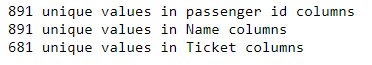

891 unique values in passenger id and name columns

乘客ID和名称列中的891个唯一值

681 unique values in ticket columns.

凭单列中有681个唯一值。

So , These three columns will not be do any effect on our prediction. these columns not useful, because all values are unique values .so we are dropping these three columns from the dataset.

因此，这三列将不会对我们的预测产生任何影响。 这些列没有用，因为所有值都是唯一值。因此我们从数据集中删除了这三列 。

STEP 7- Drop these three columns

步骤7-删除这三列

data=data.drop(['PassengerId','Name','Ticket'],axis=1)

STEP 8-

步骤8

data.shape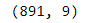

Check the shape of dataframe once again .It has 891 *9.

再次检查数据框的形状。它具有891 * 9。

Now, After drop three features .9 columns (features) present in dataset.

现在，删除三个功能。 数据集中存在9列 ( 特征 )。

STEP 9 - In this step, we gonna go check is this dataset is balance or not.

步骤9-在这一步中 ，我们将检查此数据集是否平衡。

If dataset is not balance . it might be reason of bad accuracy, because in dataset. if you have many data points which belong only to single class. so this thing may lead over-fitting problem.

如果数据集不平衡。 这可能是因为数据集中的准确性不佳 。 如果您有许多仅属于单个类的数据点。 所以这东西可能会导致过度拟合的问题。

data["Survived"].value_counts().plot(kind='bar')

Here, Dataset is not proper balance, it’s 60–40 ratio.

这里 ，数据集不是适当的平衡， 它是60–40的比率。

So , it will not be effect so much on our predictions. If it effect on our prediction we will deal with this soon.

因此，它对我们的预测影响不大。 如果它影响我们的预测， 我们将尽快处理。

STEP 10 -

步骤10-

datasett=data.copynot_survived=data[data['Survived']==0]survived=data[data['Survived']==1]

1st line of code — Copy the dataset in dataset variable. because , we will perform some manipulation on data . so that manipulation does not effect on real data. so that we are copying dataset into datasett variable.

第一行代码—将数据集复制到数据集变量中。 因为，我们将对数据进行一些处理 。 这样操作就不会影响真实数据。 所以，我们要复制的数据集到datasett变量。

2nd line of code - we are dividing dependent feature (“Survived “) into two part-

代码的第二行-我们将依存特征(“幸存的”)分为两部分，

1. extract all non survival data points from the “Survived” column and store into not_survived variable.

1.从“生存”列中提取所有非生存数据点，并将其存储到not_survived变量中。

2. extract all survival data points from the “Survived” column and store into survival variable.

2.从“ Survived”列中提取所有生存数据点，并将其存储到生存变量中。

It is for visualize the dataset.

用于可视化数据集。

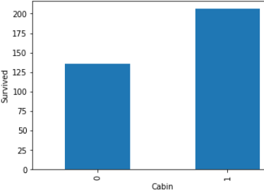
STEP 11 - Now , We are checking of null values’s features(columns) dependency with the Survived or non survived peoples .

步骤11-现在 ，我们正在与生存或未生存的人一起检查空值的特征 ( 列 ) 依赖性 。

First of all , right here, we are checking null values ‘s features(columns) dependency with survived people only.

首先，在这里，我们仅与幸存者一起检查null值的功能(列)依赖性。

import matplotlib.pyplot as pltdataset = survived.copy()%matplotlib inline for features in null_features:    dataset[features] = np.where(dataset[features].isnull(), 1, 0)    dataset.groupby(features)['Survived'].count().plot.bar()    plt.xlabel(features)    plt.ylabel('Survived')    plt.title(features)    plt.show()

1st line of code- Import matplotlib.lib for visualize purpose.

第一行代码-我导入matplotlib.lib以实现可视化目的。

2nd line of code- copy the only survived people dataset into dataset variable for further processing and it copy because any manipulation does not effect on real data frame.

代码的第二行-将唯一幸存的人员数据集复制到数据集变量中以进行进一步处理， 并进行复制，因为任何操作都不会影响实际数据帧。

3rd line of code - Used loop . This loop will take only null value’s features(columns) only.

第三行代码-使用循环 。 此循环将仅采用空值的功能(列)。

4th line of code — Null values replace by the 1 or non null values replace by 0. for check the dependency.

代码的第四行- 空值替换为1或非空值替换为0 。 用于检查依赖性 。

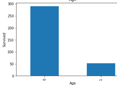
Look in above graphs . all 1 values is basically null values and 0 values is not null values.

看上面的图表 。 所有1个值基本上都是空值，而0个值不是空值。

In age’s graph , dependency is low with null value .

在age的图中，依赖性较低，值为null。

In cabin’s graph, dependency is high with null values.

在机舱的图形中，具有空值的依赖性较高。

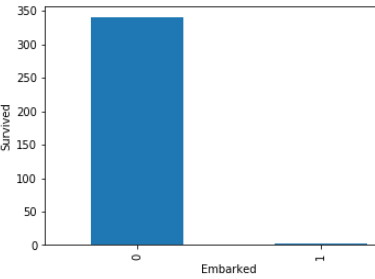
In embarked’s graph ,there is approximate not any dependency with null values.

在图的图形中，没有近似值的依赖项为空。

STEP 12- Over here, we are checking dependency with not survived peoples.

第12步-在这里， 我们正在检查对尚未幸存的民族的依赖性。

import matplotlib.pyplot as pltdataset = not_survived.copy()%matplotlib inline for features in null_features:    dataset = not_survived.copy()    dataset[features] = np.where(dataset[features].isnull(), 1, 0)    dataset.groupby(features)['Survived'].count().plot.bar()    plt.xlabel(features)    plt.ylabel('Survived')    plt.title(features)    plt.show()

Same like step 7 . but over here we are dealing with non survival people’s.

与步骤7相同。 但在这里，我们正在与非生存者打交道。

STEP 13 -Let find the relationship between all categories variable(features) with survive peoples.

步骤13-让我们找出所有类别变量 (特征)与生存人群之间的关系。

num_features=data.columnsfor feature in num_features:    if feature != 'Survived' and feature !='Fare' and feature != 'Age':        survived.groupby(feature)['Survived'].count().plot.bar()        plt.xlabel(feature)        plt.ylabel('Survived')        plt.title(feature)        plt.show()

Survived is dependent variable (feature).

生存的是因变量(特征)。

Fare is numeric variable.

票价是数字变量。

Age is also numeric variable.

年龄也是数字变量。

So , we are not considering these three features (columns) .

因此 ，我们不考虑这三个功能 ( 列 )。

These all are relationship between categorical variables(features) with survived peoples.

这些都是类别变量 ( 特征 )与幸存者之间的关系 。

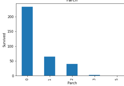
STEP 14- Let find the relationship between all categories variable with not survived peoples.

步骤14-让所有类别的变量与没有生存的人之间建立关系 。

for feature in num_features:    if feature != 'Survived' and feature !='Fare' and feature != 'Age':        not_survived.groupby(feature)['Survived'].count().plot.bar()        plt.xlabel(feature)        plt.ylabel('Not Survived')        plt.title(feature)        plt.show()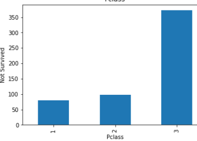

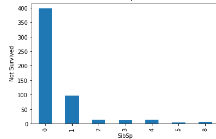
These all are relationship between categorical variables(features) with not survived peoples.

这些都是没有生存的人的 分类变量 ( 特征 )之间的关系 。

STEP 15 -Now check with the numeric variables.

步骤15-现在检查数字变量 。

non_sur_fare_mean=round(not_survived['Fare'].mean())non_sur_age_mean=round(not_survived['Age'].mean())  print('its not survived people fare averages',non_sur_fare_mean)print('its not survived people Age averages',non_sur_age_mean)sur_fare_mean=round(survived['Fare'].mean())sur_age_mean=round(survived['Age'].mean())  print('its survived people fare averages',sur_fare_mean)print('its survived people Age averages',sur_age_mean)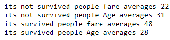

From this , Its clearly show-

由此可见，它清楚地表明：

Those who were above 31 years old had very few chances to escapes.

那些31岁以上的人很少有机会逃脱。

Those who fares was less than 48 had very few chances to escapes.

票价低于48美元的人几乎没有机会逃脱。

STEP 16- Analysis the numeric features. check distribution of the numeric variable(features).

步骤16- 分析 数字特征 。 检查数字变量的 分布 ( 功能 )。

for feature in num_features:    if feature =='Fare' or feature == 'Age':        data[feature].hist(bins=25)        plt.xlabel(feature)        plt.ylabel("Count")        plt.title(feature)        plt.show()

Age followed normal distribution, but Fare is not following normal distribution.

年龄遵循正态分布 ，但票价不遵循正态分布 。

STEP 17- Check the outliers in dataset.

步骤17-检查数据集中的离群值 。

There are many ways to check the outliers.

有许多方法可以检查异常值。

1- Box plot.

1-盒图。

2- Z-score.

2-Z得分。

3- scatter plot

3-散点图

ETC.

等等。

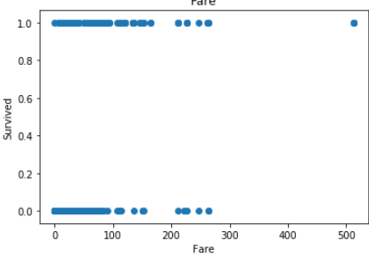
First of all , Find the outliers using scatter plot-

首先，使用散点图找到离群值-

for feature in num_features:        if feature =='Fare' or feature == 'Age':plt.scatter(data[feature],data['Survived'])                plt.xlabel(feature)                plt.ylabel('Survived')                plt.title(feature)                plt.show()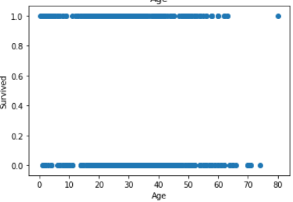

In Age less no of outlier.

在年龄中，没有异常值。

but in fare you can see there is lot of outlier in fare.

但是在票价上您可以看到票价中有很多离群值。

STEP 18- Find outlier using box plot-

步骤18- 使用箱形图查找离群值-

Box plot is better way to check outlier in distribution.

箱形图是检查分布中异常值的更好方法。

for feature in num_features:    if feature =='Fare' or feature == 'Age':            data.boxplot(column=feature)            plt.ylabel(feature)            plt.title(feature)            plt.show()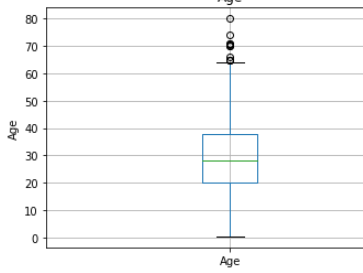

Box plot is also show same picture like scatter.

箱形图也显示散点图。

Age has few no of outlier , but in fare has lot of outliers.

年龄很少有异常值，但票价中有很多异常值。

This first part ended here.

第一部分到此结束。

In this part we saw. how, we can analysis and visualize the dataset.

在这一部分中，我们看到了。 如何分析和可视化数据集。

In next part we will see how feature engineering perform.

在下一部分中，我们将了解要素工程的性能。