A single-cell map of intratumoral changes during anti-PD1 treatment of patients with breast cancer

https://doi.org/10.1038/s41591-021-01323-8

文章目录

A single-cell map of intratumoral changes during anti-PD1 treatment of patients with breast cancer
前言
讲在前面的废话
文章导读
图表复现
- Step.00 Download_Data
- Step.01 Create Seurat obj for Cohort1
- Step.02 Data clean & Standerdize processing
- Step.03 Cell Annotion
- Step.04 Cancer cell detection
- - BscModel
  - InferCNV

前言

Seurat-单细胞文献复现第二弹-01
Seurat-单细胞文献复现第二弹-02

讲在前面的废话

文章是一个好文章，但是没给代码，这一点就要差评

文章导读

Motivation：

To understand why only a subset of tumors respond to ICB（想了解一下免疫治疗耐受的原因）

Data：

one cohort of patients with non-metastatic, treatment-naive primary invasive carcinoma of the breast was treated with one dose of pembrolizumab (Keytruda or anti-PD1) approximately 9 ± 2 days before surgery (Fig. 1a and Methods). A second cohort of patients received neoadjuvant che- motherapy for 20–24 weeks, which was followed by pembrolizumab before surgery.
（一共两个队列，都是配套的数据，PD-L1 治疗前后的单细胞测序和 TCR）

图表复现

fig1 和配套的补充材料

Step.00 Download_Data

数据太大了，没办法从头处理，只能直接使用文献提供的数据，因为提供的是 rds 的文件，所以需要一些处理

a download of the read count data per individual patient
is publicly available at
http://biokey.lambrechtslab.org.

Convert sparse matrix to count matrix

# optionss
rm(list=ls())
gc()
options(stringsAsFactors = F)
options(as.is = T)# packages
library(stringr)
library(magrittr)
library(Seurat)# my_function
as_matrix <- function(mat){tmp <- matrix(data=0L, nrow = mat@Dim[1], ncol = mat@Dim[2])row_pos <- mat@i+1col_pos <- findInterval(seq(mat@x)-1,mat@p[-1])+1val <- mat@xfor (i in seq_along(val)){tmp[row_pos[i],col_pos[i]] <- val[i]}row.names(tmp) <- mat@Dimnames[[1]]colnames(tmp) <- mat@Dimnames[[2]]return(tmp)
}# load data
if(F){cohort1 = readRDS("../rawdata/1863-counts_cells_cohort1.rds")df1 = as_matrix(cohort1)cohort2 = readRDS("../rawdata/1867-counts_cells_cohort2.rds")df2 = as_matrix(cohort2)save(df1,df2,file = '../rawdata/cohort1_and_cohort2.rdata')
}

首先第一步就是获取 Seurat 对象，这一部分文章只用了 cohor1的队列

Step.01 Create Seurat obj for Cohort1

# options
rm(list=ls())
gc()
options(stringsAsFactors = F)
options(as.is = T)# packages
library(stringr)
library(magrittr)
library(Seurat)# set work-dir
setwd('/Yours')# load data
load("Count/cohort1_and_cohort2.rdata")
predict = read.csv('output/raw_predict-Cohort1.csv',row.names = 1)
meta = read.csv('Count/1872-BIOKEY_metaData_cohort1_web.csv',row.names = 1)
rm(df2)
gc()
ids = predict %>% rownames()
meta$CellType = ifelse(rownames(meta) %in% ids,predict$label,meta$cellType)# Create Seurat obj
sce = CreateSeuratObject(counts = df1)
sce = AddMetaData(sce, metadata = meta)
save(sce,file='output/cohort1_sce.rdata')

Step.02 Data clean & Standerdize processing

根据文章在 Method 中的信息进行数据处理

All cells expressing <200 or >6,000 genes were removed, as well as cells that contained <400 unique molecular identifiers (UMIs) and >15% mitochondrial counts.

数据中是没有 UMI 信息的

# options
rm(list=ls())
gc()
options(stringsAsFactors = F)
options(as.is = T)# packages
library(stringr)
library(magrittr)
library(Seurat)# set work-dir
setwd('/Yours')# load data
load('output/cohort1_sce.rdata')
tcr = read.csv('scTCR/1879-BIOKEY_barcodes_vdj_combined_cohort1.csv')
tcr.info = read.csv('scTCR/1881-BIOKEY_clonotypes_combined_cohort1.csv')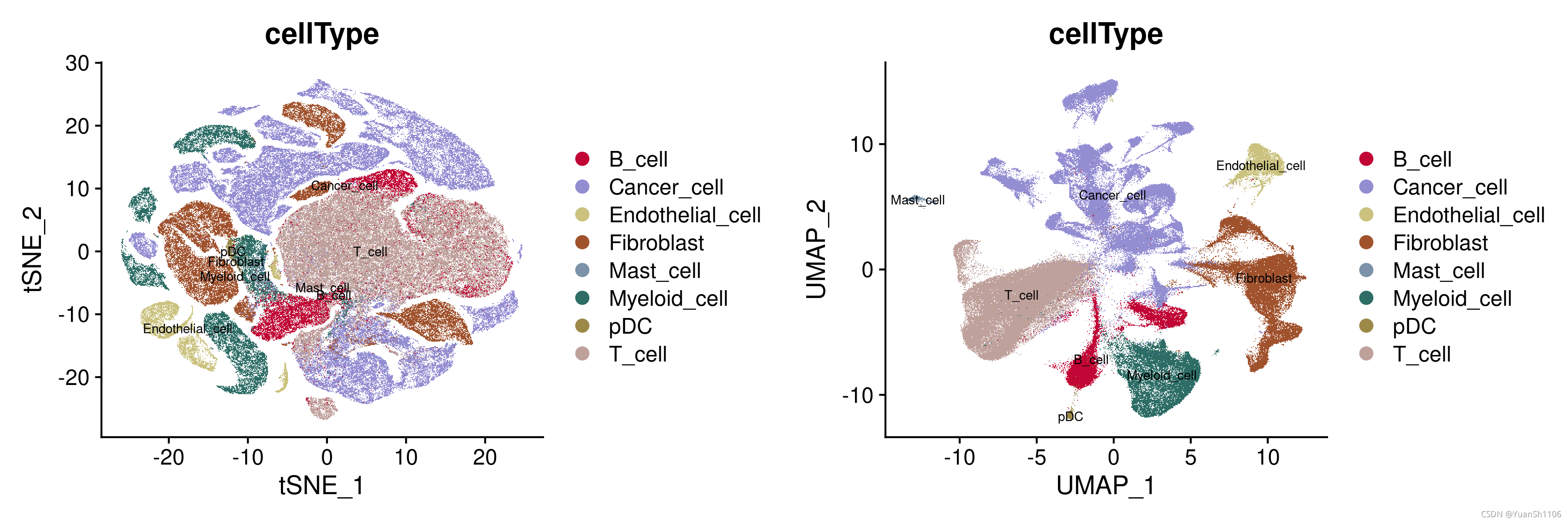![请添加图片描述](https://img-blog.csdnimg.cn/323c827b6a8243dd98dd6a5e1816ad68.png?x-oss-process=image/watermark,type_ZHJvaWRzYW5zZmFsbGJhY2s,shadow_50,text_Q1NETiBAWXVhblNoMTEwNg==,size_20,color_FFFFFF,t_70,g_se,x_16)# my functions
# mycolors = stata_pal("s2color")(15)
mycolors = c("#1a476f","#90353b","#55752f","#e37e00","#6e8e84","#c10534","#938dd2","#cac27e","#a0522d","#7b92a8","#2d6d66","#9c8847","#bfa19c","#ffd200","#d9e6eb")# clean
# 1. All cells expressing <200 or >6,000 genes
# 2. <400 unique molecular identifiers (UMIs)
# 3. >15% mitochondrial counts.
mt = grep('^MT-', x= rownames(sce),value = T)
sce[["percent.mt"]]  = PercentageFeatureSet(sce, pattern = "^MT-")# 1.log
sce = NormalizeData(object = sce,normalization.method =  "LogNormalize",  scale.factor = 1e4)
# 2.FindVariable
sce = FindVariableFeatures(object = sce,selection.method = "vst", nfeatures = 2000)
# 3.ScaleData
sce = ScaleData(object = sce)
# 4. PCA
sce = RunPCA(object = sce, do.print = FALSE)
# 5.Neighbor
sce= FindNeighbors(sce, dims = 1:20)
# 6. Clusters
sce = FindClusters(sce, resolution = 0.5)
# 7.tsne
sce=RunTSNE(sce,dims.use = 1:20)
# 8.plot
p1 = DimPlot(sce,reduction = "tsne",label=T, group.by = "cellType",cols=mycolors[6:15],label.size=2.5)
p2 = DimPlot(sce,reduction = "umap",label=T, group.by = "cellType",cols=mycolors[6:15],label.size=2.5)
CombinePlots(plots =list(p1, p2))
ggsave('plot/Cohort1_CellType_plot.png', width = 12, height = 4)

经过检查发现数据是经过过滤的，所以不需要进行过滤操作，直接跑流程就行。

由于文章没有给出明确的参数，所以这里只能按照标准流程跑了

分群后使用原文的标签进行可视化评估，从图中可以看出来，分群的结果还可以（UMAP），各个细胞的分群边界比较清晰。

验证一下原始文献的注释结果，从UMAP的结果可以看出，不同的细胞类型离散程度较高

Step.03 Cell Annotion

根据文章补充材料的基因 marker 进行注释。
有一点值得注意一下，
这篇文章不是根据 epcam 进行肿瘤细胞定义的，然后我自己去用 epcam 评估过后发现这部分的 epcam 表达丰度很低
并且使用 BscModel 评估后发现，这部分的肿瘤候选细胞纯度很高，还是比较可信的

Next, we annotate cells using genes in artical

# get gene list
gene.list = c('CD3D','CD3E','CD2','COL1A1','DCN','C1R','LYZ','CD68','TYROBP','CD24','KRT19','SCGB2A2','CD79A','MZB1','MS4A1','CLDN5','FLT1','RAMP2','CPA3','TPSAB1','TPSB2','LILRA4','CXCR3','IRF7')
FeaturePlot(object = sce, features=gene.list)
p = DotPlot(sce, features = gene.list) + coord_flip()
p
ggsave('plot/Cell_annotion_DotPlot.png', width = 10, height = 10)

细胞群落的基因表达丰度图

根据原文的基因集，查看不同细胞群落的特意基因表达情况

细胞注释流程

由于这部分的细胞分群太多，而且基因也很多，一个个看过去眼睛会瞎掉，所以先进行粗注释然后在进行细注释

### Cell Markers
T.cell.marker = c("CD3D",'CD3E','CD2')
Fib.cell.marker = c('COL1A1','DCN','C1R')
Myeioid.cell.marker = c('LYZ','CD68','TYROBP')
Cancer.cell.marker = c('CD24','KRT19','SCGB2A2')
B.cell.marker= c('CD79A','MZB1','MS4A1')
Endothelial.cell.marker= c('CLDN5','FLT1','RAMP2')
Mast.cell.marker= c('CPA3','TPSAB1','TPSB2')
DC.cell.marker= c('LILRA4','CXCR3','IRF7')### Define CellType
cell_type = c('T-cell','Fibroblast','Myeloid cell','Cancer cell','B-cell','Endothelial cell','Mast cell',"pDC")
markers = c("T.cell.marker","Fib.cell.marker","Myeioid.cell.marker","Cancer.cell.marker", "B.cell.marker","Endothelial.cell.marker", "Mast.cell.marker","DC.cell.marker")# Cell types were preliminarily identified according to expression levels
for(i in 1:length(cell_type)){p = DotPlot(sce, features = get(markers[i])) + coord_flip()ids = as.numeric(p$data[which(p$data$avg.exp.scaled > 0 ),]$id)-1ids = table(ids)[which(table(ids) >=2)] %>% names() %>% as.numeric()ids = rownames(sce@meta.data[which(sce@meta.data$seurat_clusters %in% ids),])assign(cell_type[i], ids)
}
length(c(get(cell_type[1]),get(cell_type[2]),get(cell_type[3]),get(cell_type[4]),get(cell_type[5]),get(cell_type[6]),get(cell_type[7]),get(cell_type[8])))
ids = unique(c(get(cell_type[1]),get(cell_type[2]),get(cell_type[3]),get(cell_type[4]),get(cell_type[5]),get(cell_type[6]),get(cell_type[7]),get(cell_type[8])))
rest = setdiff(rownames(sce@meta.data),ids)
sce@meta.data$cell_annotion = ifelse(rownames(sce@meta.data) %in% get(cell_type[1]),cell_type[1],ifelse(rownames(sce@meta.data) %in% get(cell_type[2]),cell_type[2],ifelse(rownames(sce@meta.data) %in% get(cell_type[3]),cell_type[3],ifelse(rownames(sce@meta.data) %in% get(cell_type[4]),cell_type[4],ifelse(rownames(sce@meta.data) %in% get(cell_type[5]),cell_type[5],ifelse(rownames(sce@meta.data) %in% get(cell_type[6]),cell_type[6],ifelse(rownames(sce@meta.data) %in% get(cell_type[7]),cell_type[7],ifelse(rownames(sce@meta.data) %in% get(cell_type[8]),cell_type[8],'rest'))))))))### Check Unique & consistency
check.unique = NULL
for(i in 1:7){for(j in (i+1):8){len = intersect(get(cell_type[i]),get(cell_type[j]))if(length(len) != 0 ){ids = c(cell_type[i],cell_type[j],markers[i],markers[j],length(len))check.unique = rbind(check.unique,ids)}}
}
check.unique##### Manual Adjust
i=5 # for i in 1:dim(check.unique)[1]
ids1 = check.unique[i,1]
ids2 = check.unique[i,2]
gen1 = check.unique[i,3]
gen2 = check.unique[i,4]
ids = intersect(get(ids1),get(ids2))
DotPlot(sce[,ids], features = c(get(gen1),get(gen2)))  + coord_flip()
ids1
ids2
DotPlot(sce[,rest], features =gene.list)  + coord_flip()
DotPlot(sce, features =c(get('B.cell.marker'),get('Cancer.cell.marker')))   + coord_flip()sce@meta.data[which(sce@meta.data$seurat_clusters == 19),'cell_annotion'] = "T-cell"
sce@meta.data[which(sce@meta.data$seurat_clusters == 1),'cell_annotion'] = "T-cell"
sce@meta.data[which(sce@meta.data$seurat_clusters == 6),'cell_annotion'] = "T-cell"
sce@meta.data[which(sce@meta.data$seurat_clusters == 33),'cell_annotion'] = "Fibroblast"
sce@meta.data[which(sce@meta.data$seurat_clusters == 30),'cell_annotion'] = "Fibroblast"
sce@meta.data[which(sce@meta.data$seurat_clusters == 8),'cell_annotion'] = "Cancer cell"
sce@meta.data[which(sce@meta.data$seurat_clusters == 23),'cell_annotion'] = "Cancer cell"
sce@meta.data[which(sce@meta.data$seurat_clusters == 24),'cell_annotion'] = "Cancer cell"
sce@meta.data[which(sce@meta.data$seurat_clusters == 18),'cell_annotion'] = "Cancer cell"
sce@meta.data[which(sce@meta.data$seurat_clusters == 29),'cell_annotion'] = "pDC"##### consistency
sce@meta.data$cell_annotion = str_replace_all(sce@meta.data$cell_annotion, c("B-cell" = "B_cell","Cancer cell" = "Cancer_cell","Endothelial cell" = "Endothelial_cell","Fibroblast" = "Fibroblast","Mast cell" = "Mast_cell","Myeloid cell" = "Myeloid_cell","pDC" = "pDC","T-cell" = "T_cell"))### plot
p1 = DimPlot(sce,reduction = "tsne",label=T, group.by = "cell_annotion",cols=mycolors[6:15],label.size=2.5)
p2 = DimPlot(sce,reduction = "umap",label=T, group.by = "cell_annotion",cols=mycolors[6:15],label.size=2.5)
CombinePlots(plots =list(p1, p2))
ggsave('plot/Cohort1_cell_annotion_plot.png', width = 12, height = 4)

自己的分群结果，与原文的一致性97.26%

Marker gene 热图

### plot
p1 = DimPlot(sce,reduction = "tsne",label=T, group.by = "cell_annotion",cols=mycolors[6:15],label.size=2.5)
p2 = DimPlot(sce,reduction = "umap",label=T, group.by = "cell_annotion",cols=mycolors[6:15],label.size=2.5)
CombinePlots(plots =list(p1, p2))
ggsave('plot/Cohort1_cell_annotion_plot.png', width = 12, height = 4)# cell type heat-map
for(i in 1:length(gene.list)){ids = sce[gene.list[i],]ids = ids@assays$RNA@data %>% as.numeric()assign(gene.list[i],tapply(ids, sce@meta.data$cell_annotion,mean))
}heatmap_matrix = NULL
for (i in 1:length(gene.list)) {heatmap_matrix = rbind(heatmap_matrix,get(gene.list[i]))
}
row.names(heatmap_matrix) = gene.list
ids = c("T_cell","Fibroblast","Myeloid_cell","Cancer_cell","B_cell","Endothelial_cell","Mast_cell","pDC")
heatmap_matrix = heatmap_matrix[,ids]
pheatmap::pheatmap(heatmap_matrix,scale = 'row',cluster_cols = F,cluster_rows = F,filename = 'plot/Cohort1_cell_annotion_hm.png')
meta = sce@meta.data

这个和原文基本上完全一样，可以自行对比

治疗前后细胞比例变化

# NE / E
names(table(meta$patient_id))
ids = c(7,9,18,20,4,13,19,22,23,26,29,30,21,28,31,11,5,17,27,6,12,16,10,3,8,25,14,24,2)
ids = paste0('BIOKEY','_',ids)
meta = meta[which(meta$patient_id %in% ids),]
E = c('BIOKEY_12','BIOKEY_16','BIOKEY_10','BIOKEY_3','BIOKEY_8','BIOKEY_25','BIOKEY_14','BIOKEY_24','BIOKEY_2')
meta$Ne_type = ifelse(meta$patient_id %in% E,'E','NEs')# pre- / on- cell rations
pre = meta[which(meta$timepoint == 'Pre'),]
on = meta[which(meta$timepoint == 'On'),]
ids1 = table(pre$cell_annotion) %>% as.data.frame()
ids2 = table(on$cell_annotion) %>% as.data.frame()
ids1$group = 'pre'
ids2$group = 'on'
df = rbind(ids1,ids2)ggplot(data=df, mapping=aes(x=Freq,y=Var1,fill=group))+geom_bar(stat='identity',width=0.5,position='fill')+theme_bw()+scale_fill_manual(values = mycolors[7:6])+geom_vline(aes(xintercept=0.48),color = 'black',linetype='dashed')
ggsave('plot/Cohort1_cell_ratio_bar_plot.png', width = 6.7, height = 7.6)

NE / Es 的变化

df = pre
ids = table(df$patient_id) %>% as.data.frame()
df.plot = table(df[,c('patient_id','cell_annotion')]) %>% as.data.frame()
df.plot$prop = 0
for(i in 1:dim(ids)[1]){prop.temp = df.plot[which(df.plot$patient_id %in% ids[i,1]),'Freq'] / ids[i,2]df.plot[which(df.plot$patient_id %in% ids[i,1]),'prop'] = prop.temp
}
df.plot$cell_annotion = factor(df.plot$cell_annotion,levels = c("T_cell","Fibroblast","Myeloid_cell","Cancer_cell","B_cell","Endothelial_cell","Mast_cell","pDC"))
df.plot$Ne_type = ifelse(df.plot$patient_id %in% E,'E','NEs')
df.plot$Ne_type = factor(df.plot$Ne_type,levels = c('NEs','E'))
df.plot
ggplot(data=df.plot, mapping=aes(x=cell_annotion,y=prop,color=Ne_type))+geom_boxplot()+theme_bw()+scale_color_manual(values = mycolors[7:6])
ggsave('plot/Cohort1_pre_box_plot.png', width = 8.24, height = 2.84)df = on
ids = table(df$patient_id) %>% as.data.frame()
df.plot = table(df[,c('patient_id','cell_annotion')]) %>% as.data.frame()
df.plot$prop = 0
for(i in 1:dim(ids)[1]){prop.temp = df.plot[which(df.plot$patient_id %in% ids[i,1]),'Freq'] / ids[i,2]df.plot[which(df.plot$patient_id %in% ids[i,1]),'prop'] = prop.temp
}
df.plot$cell_annotion = factor(df.plot$cell_annotion,levels = c("T_cell","Fibroblast","Myeloid_cell","Cancer_cell","B_cell","Endothelial_cell","Mast_cell","pDC"))
df.plot$Ne_type = ifelse(df.plot$patient_id %in% E,'E','NEs')
df.plot$Ne_type = factor(df.plot$Ne_type,levels = c('NEs','E'))
df.plot
ggplot(data=df.plot, mapping=aes(x=cell_annotion,y=prop,color=Ne_type))+geom_boxplot()+theme_bw()+scale_color_manual(values = mycolors[7:6])
ggsave('plot/Cohort1_on_box_plot.png', width = 8.24, height = 2.84)

Step.04 Cancer cell detection

BscModel

First, get logNormalize data and the follow the document of BscModel to set config

# cohort1
sce = CreateSeuratObject(counts = df1)
sce = AddMetaData(sce, metadata = sd1)
sce <- NormalizeData(object = sce, scale.factor = 1e6)
use.cells = sce@meta.data[which(sce@meta.data$cellType == 'Cancer_cell'),] %>% rownames()
sce = subset(sce,cells = use.cells)
df = sce@assays$RNA@data %>% as.data.frame()
max(df)
min(df)
write.csv(df,'../processfile/Cohort1_epi_expr.csv')# cohort2
sce = CreateSeuratObject(counts = df2)
sce = AddMetaData(sce, metadata = sd2)
sce <- NormalizeData(object = sce, scale.factor = 1e6)
use.cells = sce@meta.data[which(sce@meta.data$cellType == 'Cancer_cell'),] %>% rownames()
sce = subset(sce,cells = use.cells)
df = sce@assays$RNA@data %>% as.data.frame()
max(df)
min(df)
write.csv(df,'../processfile/Cohort2_epi_expr.csv')

Then, run the script

python main.py --config configs/Training_and_predict.yaml

InferCNV

Prepare file & Run

# main
# 导入原始表达矩阵
# main
# 导入原始表达矩阵
if(T){load("./rawdata/cohort1_and_cohort2.rdata")rm(df2)gc()info = read.csv('processfile/predict-Cohort1.csv',row.names = 1)info = info[which(info$label!='Moderate'),]#use.cell = info$Xmeta = read.csv('rawdata/1872-BIOKEY_metaData_cohort1_web.csv',row.names = 1)meta$cellType = ifelse(rownames(meta) %in% rownames(info),info$label,meta$cellType)
}
meta[which(meta$cellType == 'Cancer_cell'),'cellType'] = 'Moderate'
info = meta
a = names(table(info$cellType))
for(i in a){print(i)}use.cell = c("Endothelial_cell","Fibroblast","Moderate","Normal","Tumor")use.cell = c("B_cell","Mast_cell","Moderate","Myeloid_cell","Normal","pDC","T_cell","Tumor")
use.cell = info[which(info$cellType %in% use.cell),] %>% rownames()
#df2 = df2[,use.cell]
df1 = df1[,use.cell]
info = info[use.cell,]if(T){# 第一个文件count矩阵dfcount = df1# 第二个文件样本信息矩阵groupinfo= data.frame(cellId = colnames(dfcount))identical(groupinfo[,1],rownames(info))groupinfo$cellType = info$cellType# 第三文件library(AnnoProbe)geneInfor=annoGene(rownames(dfcount),"SYMBOL",'human')geneInfor=geneInfor[with(geneInfor, order(chr, start)),c(1,4:6)]geneInfor=geneInfor[!duplicated(geneInfor[,1]),]## 这里可以去除性染色体# 也可以把染色体排序方式改变dfcount =dfcount [rownames(dfcount ) %in% geneInfor[,1],]dfcount =dfcount [match( geneInfor[,1], rownames(dfcount) ),] myhead(dfcount)myhead(geneInfor)myhead(groupinfo)# 输出expFile='./processfile/88284_expFile.txt'write.table(dfcount ,file = expFile,sep = '\t',quote = F)groupFiles='./processfile/88284_groupFiles.txt'write.table(groupinfo,file = groupFiles,sep = '\t',quote = F,col.names = F,row.names = F)geneFile='./processfile/88284_geneFile.txt'write.table(geneInfor,file = geneFile,sep = '\t',quote = F,col.names = F,row.names = F)
}
# infercnv流程
a = names(table(groupinfo$cellType))
for(i in a){print(i)}if(T){rm(list=ls())setwd('/media/yuansh/14THHD/胶囊单细胞/测试集/EGAD/')options(stringsAsFactors = F)library(Seurat)library(ggplot2)library(infercnv)expFile='./processfile/88284_expFile.txt' groupFiles='./processfile/88284_groupFiles.txt'  geneFile='./processfile/88284_geneFile.txt'library(infercnv)infercnv_obj = CreateInfercnvObject(raw_counts_matrix=expFile,annotations_file=groupFiles,delim="\t",gene_order_file= geneFile,ref_group_names=c("Endothelial_cell","Fibroblast")) # 如果有正常细胞的话，把正常细胞的分组填进去library(future)plan("multiprocess", workers = 16)infercnv_all = infercnv::run(infercnv_obj,cutoff=0.1,  # use 1 for smart-seq, 0.1 for 10x-genomicsout_dir= "./processfile/88284_inferCNV_Cohort1",  # dir is auto-created for storing outputscluster_by_groups=T,   # clusternum_threads=32,denoise=F,HMM=F)
}

这里展示的是 Cohort2 数据，因此图和原文有差异

### ---------------
###
### Create: Yuan.Sh
### Date: 2021-10-14 23:52:41
### Email: yuansh3354@163.com
### Blog: https://blog.csdn.net/qq_40966210
### Fujian Medical University
###
### ---------------> 课题项目合作以及咨询请联系：yuansh3354@163.comAfter advisement, if you still have questions, you can send me an E-mail asking for help
Best Regards,
Yuan.SH
---------------------------------------
please contact me via the following ways:
(a) E-mail: yuansh3354@gmail/163/outlook.com
(b) QQ: 1044532817
(c) WeChat: YuanSh181014
(d) Address: School of Basic Medical Sciences,
Fujian Medical University, Fuzhou,
Fujian 350108, China
---------------------------------------

Seurat-单细胞文献复现第二弹-01相关推荐

Seurat-单细胞文献复现第二弹-02
A single-cell map of intratumoral changes during anti-PD1 treatment of patients with breast cancer h ...
（单细胞-SingleCell）Seurat流程文献复现——单细胞实战分析流程
单细胞项目:来自于30个病人的49个组织样品,跨越3个治疗阶段 Therapy-Induced Evolution of Human Lung Cancer Revealed by Single-Ce ...
翻车实录之Nature Medicine新冠单细胞文献|附全代码
前言 NGS系列文章包括NGS基础.转录组分析 (Nature重磅综述|关于RNA-seq你想知道的全在这).ChIP-seq分析 (ChIP-seq基本分析流程).单细胞测序分析 (重磅综述:三万字 ...
Android ANR 问题第二弹------Input超时实战问题解析上
在前面的Android ANR 问题第二弹一文中,我们简诉了Android Input超时的原因,我们了解到系统Input系统分发Input的事件时如果有5s超时会触发应用ANR.在实际开发测试中,我 ...
培训第二弹：全国大学生智能汽车竞赛百度竞速组预告
§01 竞赛培训 3月12日本周六晚7点,百度飞桨B站直播间,第十七届全国大学生智能汽车竞赛完全模型组竞速赛第二次线上培训正式开讲! ▲ 图1 卓老师前来百度科技园"检查作业" ▲ ...
青瓷引擎之纯JavaScript打造HTML5游戏第二弹——《跳跃的方块》Part 3
继上一次介绍了<神奇的六边形>的完整游戏开发流程后(可点击这里查看),这次将为大家介绍另外一款魔性游戏<跳跃的方块>的完整开发流程. (点击图片可进入游戏体验) 因内容太多,为 ...
浅谈Hybrid技术的设计与实现第二弹
前言浅谈Hybrid技术的设计与实现浅谈Hybrid技术的设计与实现第二弹浅谈Hybrid技术的设计与实现第三弹--落地篇接上文:浅谈Hybrid技术的设计与实现(阅读本文前,建议阅读这个先) ...
【文献复现】-氧还原反应塔菲尔斜率绘制(文献阅读)
氧还原反应塔菲尔斜率绘制氧还原反应模型模型复现本文主要是记录文献阅读与文献复现的内容,所阅读的文献为:Shinagawa_2015_Nature_Insight on Tafel slopes ...
一级化学反应多步骤Fluent仿真文献复现（三维、多孔介质催化剂表面反应）
个人觉得化学反应在COMSOL里面的设置是比较简单直接的,但在Fluent里面就显得复杂挺多,在此记录下本人在文献复现的思路和软件的设置过程,关于文献中的方程组,在此先不做深入的考究. 参考文献:10 ...

Seurat-单细胞文献复现第二弹-01