介绍 (Introduction)

In my previous article on the seismic bumps dataset sourced from UCI’s Data Archive, I applied basic data analysis techniques for feature engineering and test-train splitting strategies for imbalanced datasets. In this article, I have demonstrated how to apply supervised machine learning algorithms (KNN, Random Forest, and SVM) for predictions and tune hyperparameters (using GridSearchCV) for optimum results. The outcomes of the performance assessment also clearly exhibit Accuracy Paradox which I will elaborate on in the following sections. Additionally, it also demonstrates why understanding the “business problem” is essential to pick the best model.

在我以前关于UCI数据档案库中的地震颠簸数据集的文章中 ，我将基本数据分析技术应用于特征工程和不平衡数据集的测试序列拆分策略。 在本文中，我演示了如何将监督式机器学习算法(KNN，Random Forest和SVM)用于预测，以及如何调整超参数(使用GridSearchCV)以获得最佳结果。 绩效评估的结果也清楚地显示了“ 准确性悖论” ，我将在以下各节中详细阐述。 此外，它还说明了为什么理解“业务问题”对于选择最佳模型至关重要 。

The complete notebook can be found in my GitHub repository

完整的笔记本可以在我的GitHub存储库中找到

我从...开始 (I started with…)

creating a folder in which I’d save my models. When fitting multiple algorithms to your data, it is always good to save your models after training and tuning. For this, I created a folder using the datetime python module.

创建一个用于保存模型的文件夹。 当对数据拟合多种算法时，在训练和调整后保存模型总是好的。 为此，我使用datetime python模块创建了一个文件夹。

import datetimedef model_store_location():return "model-store-{}".format(datetime.date.today())model_store_location = model_store_location()print(model_store_location)!mkdir {model_store_location}

Every best performing model will be stored in this folder.

每个性能最好的模型都将存储在此文件夹中。

接下来，我建立了基准 (Next, I established a baseline)

This is a binary classification task and I selected the simplest classification model, K-Nearest Neighbours (KNN) to begin prediction modelling. KNN is one of the simplest classifiers that assign a label to the unseen instance based on the maximum number of labels in the top K similar seen instances.

这是一个二进制分类任务，我选择了最简单的分类模型K最近邻居(KNN)开始进行预测建模。 KNN是最简单的分类器之一，它基于前K个相似实例中的最大标签数，将标签分配给未见实例。

To improve models, a baseline is required, to which the subsequent models will be compared. Consequently, it is called the “Baseline Model”. Therefore, for a baseline model, I initialised a KNN classifier with default parameters:

为了改进模型，需要一个基线，随后的模型将与之进行比较。 因此，它被称为“ 基准模型 ”。 因此，对于基线模型，我使用默认参数初始化了KNN分类器：

model = KNeighborsClassifier()

Next, I checked the performance first, using StratifiedKFold of 10 splits, keeping the scoring metric ‘accuracy’.

接下来，我首先使用StratifiedKFold(分为10个部分)检查了性能，并保持了评分指标“准确性”。

skf = StratifiedKFold(n_splits=10)

For all the folds, the accuracy lies in between 0.92 to 0.93 and that closeness of the values is exhibited through the standard deviation of the scores.

对于所有折痕，准确度都在0.92至0.93之间，并且通过得分的标准偏差显示出数值的接近性。

The accuracy is really high here. Now, let’s fit the model in our training data and check the model’s performance —

这里的准确性确实很高。 现在，让我们在训练数据中拟合模型并检查模型的性能-

model.fit(X_train, y_train)y_pred = model.predict(X_test)

I added a data frame to hold each model’s hyperparameters and performances as shown below:

我添加了一个数据框来保存每个模型的超参数和性能，如下所示：

df_results = pd.DataFrame(index = ['scoring_technique',                                    'algorithm', 'n_neighbors',                                   'weights', 'leaf_size',                                    'accuracy', 'precision',                                    'recall', 'f1-score'])

And added my baseline model’s performance:

并添加了我的基准模型的性能：

from sklearn.metrics import accuracy_score, precision_score, recall_score, f1_scoredf_results['Baseline'] = ['None', model.algorithm,                          model.n_neighbors,                           model.weights,                           model.leaf_size,                          accuracy_score(y_test, y_pred),                           precision_score(y_test, y_pred),                           recall_score(y_test, y_pred),                           f1_score(y_test, y_pred)]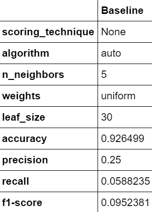

This is how the performance of KNN looks beyond accuracy. This is a classic example of an accuracy paradox. Since most the seismic bumps are non-hazardous, therefore true negatives(TN) is a much higher number than TP, FP, and FN combined, thereby numerically boosting the accuracy and creating an illusion of predictions being correct but as precision and recall show — hazardous seismic bumps identification is below 30%.

这就是KNN的性能超出准确性的样子。 这是准确性悖论的经典示例。 由于大多数地震波峰都是无害的，因此真实的负数(TN)比TP，FP和FN的总和要高得多， 因此从数字上提高了准确性，并产生了正确但对准确率和召回率的预测错觉 —危险地震波的识别率低于30％。

Binary Classification Performance Metrics —

二进制分类性能指标-

Accuracy = TP + TN / (TP + FP + TN + FN)

精度 = TP + TN /(TP + FP + TN + FN)

Precision = TP / (TP + FP)

精度 = TP /(TP + FP)

Recall = TP / (TP + FN)

召回率 = TP /(TP + FN)

F1-Score = 2 * Precision x Recall /(Precision + Recall) = 2TP/(2TP+FP+FN)

F1-分数 = 2 *精度x调用率/(精度+调用率)= 2TP /(2TP + FP + FN)

Therefore, based on the baseline performance metrics, only 25% of the predicted hazardous bumps are correct and only 5% of the actual hazardous seismic bumps were correctly identified by the model. 93% of the data actually contains non-hazardous seismic bumps and thus the accuracy figures in the cross_val_score makes sense and lies around 93% as well.

因此，基于基准性能指标，模型仅正确识别了25％的预测危险颠簸是正确的，而只有5％的实际危险地震颠簸是正确的。 93％的数据实际上包含无害的地震波，因此cross_val_score的准确度数字有意义，并且也位于93％左右。

However, as you can see, precision and recall have suffered, let’s look at tuning the hyperparameters using GridSearchCV

但是，如您所见，精度和调用率受到了影响，让我们来看一下使用GridSearchCV调整超GridSearchCV

GridSearchCV调整KNN的超参数 (GridSearchCV to Tune KNN’s Hyperparameters)

GridSearchCV is a function that takes in possible values or ranges of hyperparameters and runs all combinations of the hyperparameter values specified and calculates the performance based on the scoring metric mentioned. This scoring metric should basically align with the business value or your objectives.

GridSearchCV是一个函数，它接受可能的超参数值或范围，并运行指定的超参数值的所有组合，并根据上述评分指标计算性能。 该评分指标应基本上与业务价值或您的目标保持一致。

To see what scoring metrics are provided, this code helps:

要查看提供了哪些评分指标，此代码将帮助您：

import sklearnsorted(sklearn.metrics.SCORERS.keys())

This code will produce the entire list of scoring methods available.

此代码将生成可用的评分方法的完整列表。

Next, I defined the hyperparameters for KNN as shown in the code below, and created a dictionary called param_grid that contains the parameters for KNN’s hyperparameters, as defined in Scikit-Learns documentation on KNN, the keys, while the values contain the corresponding list of values.

接下来，我定义了KNN的超参数，如下面的代码所示，并创建了一个名为param_grid的字典，其中包含KNN的超参数的参数，如Scikit-Learns关于KNN的文档中所定义的那样 ，键是键，而值则包含对应的KNN列表。价值观。

n_neighbors = [1, 2, 3, 4, 5] weights = ['uniform', 'distance'] algorithm = ['ball_tree', 'kd_tree', 'brute'] leaf_size = [10, 20, 30 , 40, 50]  #param_grid = dict(n_neighbors=n_neighbors,                   weights=weights,                   algorithm=algorithm,                   leaf_size=leaf_size)

Next, I initialized the GridSearchCV with the model, the grid for best hyperparameter search, the cross-validation type, scoring metric as precision and I also used the refit parameter to ensure that the best-evaluated estimator is available as best_estimator_ , which is the fitted model when the training set, made available for making predictions. Verbose determines how much information you want on your screen from the logs.

接下来，我使用模型，用于最佳超参数搜索的网格，交叉验证类型，评分指标作为精度初始化GridSearchCV，并且还使用了refit参数以确保获得最佳评估的估算器为best_estimator_ ，即训练集拟合模型，可用于进行预测。 Verbose决定从日志中确定要在屏幕上显示多少信息。

grid = GridSearchCV(estimator=model,                     param_grid=param_grid,                     cv=StratifiedKFold(shuffle=True),                     scoring=['precision'],                    refit='precision',                    verbose=10)

And… I call the fit method to initiate the hyperparameter tuning process.

并且...我调用fit方法来启动超参数调整过程。

grid_result = grid.fit(X_train, y_train)

Basically, grid_result contains all the outputs, from the fit times to individual scores, and also the best model evaluated based on the passed parameters. grid_result.best_estimator_ contains the chosen values of the best-fitted model’s hyperparameters, optimized based on the scoring metric.

基本上， grid_result包含从拟合时间到单个分数的所有输出，以及基于传递的参数评估的最佳模型。 grid_result.best_estimator_包含最合适的模型超参数的选定值，这些值基于评分指标进行了优化。

I experimented with different scoring -

我尝试了不同的scoring -

Model 1 — scoring : precision

模型1- scoring ：精度

Model 2 — scoring : recall

模型2- scoring ：召回

Model 3 — scoring : f1

模型3- scoring ：f1

Following is the summary of the models’ performance:

以下是模型性能的摘要：

If you notice in this grid, the best possible outcome of scoring metrics per model belongs to that respective scoring metric specified in the entire grid, i.e., when the parameter is ‘precision’, no other model’s performance for ‘precision’ is as good as Model 1. Similarly, for ‘recall’, the best in the grid is shared by Model 2 and Model 3. In fact, their performance is the same.

如果您在此网格中注意到，则每个模型评分指标的最佳结果属于在整个网格中指定的相应scoring指标，即，当参数为“ precision”时，其他模型的“ precision”性能都不如模型1。同样，对于“召回”，模型2和模型3共享最佳网格。实际上，它们的性能是相同的。

In Model 1, whose precision is 50%, i.e. 50% of the predicted hazardous seismic bumps were correct, there is a possibility of commenting that this model is only as good as a coin toss. But the coin toss was fair while our dataset isn’t, it is an imbalanced dataset. In a fair coin toss, heads and tails are equally likely to occur but for this dataset, hazardous and non-hazardous seismic bumps are not.

在模型1中，其精度为50％，即预测的危险地震颠簸的50％是正确的，有可能评论该模型仅与抛硬币一样好。 但是抛硬币是公平的，而我们的数据集不是，这是一个不平衡的数据集。 在一次公平的抛硬币中，正面和反面同样可能发生，但对于此数据集，危险和非危险的地震颠簸不太可能发生。

In Model 2 & Model 3, recall is the highest, which can be interpreted as 14% of the actual hazardous seismic bumps that were correctly identified. The precision is 16% as well. The f1-score is far better than Model 1, which is rather good. The low f1-score of Model 1 is because of the poor recall of 2%, which says that this model could only predict 2% of the actual hazardous seismic bumps, which is no bueno.

在模型2和模型3中，召回率最高，可以解释为正确识别出的实际危险地震波的14％。 精度也是16％。 f1分数远好于Model 1，后者相当不错。 模型1的f1分数较低是因为召回率很低，仅为2％，这表示该模型只能预测实际危险地震波的2％，这不是必然的。

随机森林分类器能否赢得挑战？ (Can a Random Forest Classifier win this challenge?)

The next model that I chose is Random Forest Classifier, the competition-winning ML model. It is a robust ML model where multiple decision trees are built to ensemble their outputs. The final prediction is a function of all the individual decision tree’s predictions. This why random forest models perform better.

我选择的下一个模型是随机森林分类器，它是赢得比赛的ML模型。 这是一个健壮的ML模型，其中构建了多个决策树以整合其输出。 最终预测是所有单个决策树预测的函数。 这就是为什么随机森林模型表现更好的原因。

I started off with initializing a random forest classifier:

我从初始化随机森林分类器开始：

from sklearn.ensemble import RandomForestClassifiermodel = RandomForestClassifier()

Next, I constructed a grid to find the best-suited parameters:

接下来，我构建了一个网格以查找最适合的参数：

param_grid = { ‘bootstrap’: [True], ‘max_depth’: [80, 90, 100, 110], ‘max_features’: [2, 3, 4], ‘min_samples_leaf’: [3, 4, 5, 6], ‘min_samples_split’: [8, 10, 12], ‘n_estimators’: [100, 200, 300, 500]}

I also selected ‘precision’ again for ‘scoring’. Here is the complete code:

我还再次选择“精度”作为“得分”。 这是完整的代码：

from sklearn.ensemble import RandomForestClassifiermodel = RandomForestClassifier()param_grid = { ‘bootstrap’: [True], ‘max_depth’: [80, 90, 100, 110], ‘max_features’: [2, 3, 4], ‘min_samples_leaf’: [3, 4, 5, 6], ‘min_samples_split’: [8, 10, 12], ‘n_estimators’: [100, 200, 300, 500]}grid = GridSearchCV(estimator=model,                     param_grid=param_grid,                     cv=StratifiedKFold(shuffle=True),                     scoring=['precision'],                    refit='precision',                    verbose=10)grid_result = grid.fit(X_train, y_train)file_name = 'seismic_bump_rf_model.sav'joblib.dump(model, model_store_location + file_name)print(grid_result.best_estimator_)

The model that followed from this is —

由此产生的模型是-

However, upon predicting the test set, precision is zero.

但是，在预测测试集时，精度为零。

训练和调整支持向量机 (Training and tuning a Support Vector Machine)

Since the random forest model really disappointed me, I thought of using Support Vector Machine (SVM). SVMs belong to the kernel methods group of classification algorithms that are used to fit a decision boundary. Classification is based on which side of the decision boundary is the data-point.

由于随机森林模型确实让我感到失望，因此我想到了使用支持向量机(SVM)。 SVM属于分类算法的内核方法组，用于适应决策边界。 分类基于决策边界的哪一侧是数据点。

SVMs are computationally expensive and it can be demoed through this grid search set-up:

SVM的计算量很大，可以通过以下网格搜索设置进行演示：

from sklearn.svm import SVC model = SVC()param_grid1 = {'C': [0.1, 1, 10, 100, 1000],                'gamma': [1, 0.1, 0.01, 0.001, 0.0001],               'kernel': [ 'linear', 'poly', 'rbf', 'sigmoid']}

Fitting this grid took over 10 hours which I actually had to interrupt. I checked that a polygon kernel had better results. All linear kernels are fast but had zero precision. In total, this grid was equivalent to 500 fits, 5 folds for every 100 candidates (5 * 5 * 4).

安装此网格花费了10多个小时，实际上我不得不中断了。 我检查了多边形内核是否有更好的结果。 所有线性核都很快，但精度为零。 总体而言，此网格相当于500个拟合，每100个候选者5折(5 * 5 * 4)。

Therefore, I constructed a new grid as follows:

因此，我构建了一个新的网格，如下所示：

param_grid2 = {'C': [1],                'gamma': [1],               'kernel': ['poly', 'rbf', 'sigmoid']}

This grid had a total of 15 fits and took around 3.5 hours to complete the tuning process.

该网格总共有15个拟合，大约需要3.5个小时才能完成调整过程。

Now, following the same process, I looked at the best fitting model like below:

现在，按照相同的过程，我查看了如下的最佳拟合模型：

grid_result.best_estimator_Output:SVC(C=1, gamma=1)

The default kernel is ‘rbf’ or Radial Basis Function (RBF). To know more on kernel function, refer to Scikit-learn documentation.

默认内核是“ rbf”或径向基函数(RBF)。 要了解有关内核功能的更多信息，请参阅Scikit-learn文档 。

grid_result.best_estimator_.kernelOutput:rbf

Here is the final performance results of the SVM:

这是SVM的最终性能结果：

This looks much better in terms of precision than all the other models so far. The recall is, however, only marginally better.

就精度而言，这看起来要比到目前为止的所有其他型号好得多。 但是，召回率仅略有改善。

现在，让我们进行比较和总结... (Now, let’s compare and summarize…)

In the table above, accuracy is slightly better in the SVM but the precision has a massive improvement with 67% of the actual number of hazardous seismic bumps are being correctly predicted. However, the recall is 6%, that is, only 6% of the actual hazardous seismic bumps are correct. The f1-score of the KNN model is lower than that of SVM’s.

在上表中，SVM的准确度稍好一些，但准确预测了危险地震颠簸的实际数量的67％，因此精度有了很大提高。 但是，召回率为6％，也就是说，只有6％的实际危险地震颠簸是正确的。 KNN模型的f1得分低于SVM的f1得分。

Overall, this problem statement would require a better recall due to the risk factor associated with not being able to identify hazardous seismic bumps. The only model that performed better for the recall was KNN with uniform weights, n_neighbours as 1 and leaf_size 10.

总体而言，由于与无法识别危险的地震波峰有关的风险因素，该问题陈述将需要更好地回忆。 唯一对召回效果更好的模型是权重相同的KNN，n_neighbours为1，leaf_size为10。

The importance of business requirements varies from case to case. Sometimes recall is preferred (like here) and sometimes precision is preferred. If there is a cost associated with taking action on the predicted outcomes then precision is important, i.e., you would want less false positives. A higher recall is desired in cases when a cost is associated with every false negative. In cases, when both are important, f1-score, which is the harmonic mean of precision and recall, gets importance.

业务需求的重要性因案例而异。 有时更喜欢回忆(如此处)，有时更喜欢精确度。 如果要对预期的结果采取行动会带来成本，那么精确度就很重要，即，您需要更少的误报。 当成本与每个假阴性相关联时，需要更高的召回率。 在两种情况都很重要的情况下，f1得分(精度和召回率的谐波平均值)变得很重要。

参考： (Reference:)

[1] Sikora M., Wrobel L.: Application of rule induction algorithms for analysis of data collected by seismic hazard monitoring systems in coal mines. Archives of Mining Sciences, 55(1), 2010, 91–114.

[1] Sikora M.，Wrobel L .：规则归纳算法在分析煤矿地震灾害监测系统收集的数据中的应用。 采矿科学档案，55(1)，2010，91-114。

Thanks for visiting. I hope you enjoyed reading this blog!

感谢造访。 希望您喜欢阅读此博客！

GitHub Link to this Notebook:

GitHub链接到此笔记本：

My Links: Medium | LinkedIn | GitHub

我的链接： 中 | 领英 的GitHub