使用Numpy和Scipy处理图像

图像 = 2-D 数值数组(或者 3-D: CT, MRI, 2D + 时间; 4-D, ...)这里 图像 == Numpy数组 np.array

这个教程中使用的工具：

numpy：基本数组操作
scipy：scipy.ndimage子模块致力于图像处理(n维图像)。参见http://docs.scipy.org/doc/scipy/reference/tutorial/ndimage.html
```
from scipy import ndimage
```
一些例子用到了使用np.array的特殊的工具箱：
- Scikit Image
- scikit-learn

图像中的常见问题有：

输入/输出，呈现图像
基本操作：裁剪、翻转、旋转……
图像滤镜：消噪，锐化
图像分割：不同对应对象的像素标记

更有力和完整的模块：

OpenCV (Python绑定)
CellProfiler
ITK,Python绑定
更多……

打开和读写图像文件
呈现图像
基本操作
- 统计信息
- 几何转换
图像滤镜
- 模糊/平滑
- 锐化
- 消噪
- 数学形态学
特征提取
- 边缘检测
- 分割
测量对象属性：ndimage.measurements
Footnotes

打开和读写图像文件

将一个数组写入文件：

In [1]: from scipy import miscIn [2]: l = misc.lena()In [3]: misc.imsave('lena.png', l)  # uses the Image module (PIL)In [4]: import pylab as plIn [5]: pl.imshow(l)
Out[5]: <matplotlib.image.AxesImage at 0x4118110>

从一个图像文件创建数组：

In [7]: lena = misc.imread('lena.png')In [8]: type(lena)
Out[8]: numpy.ndarrayIn [9]: lena.shape, lena.dtype
Out[9]: ((512, 512), dtype('uint8'))

8位图像(0-255)的dtype是uint8

打开一个raw文件(相机， 3-D图像)

In [10]: l.tofile('lena.raw')  # 创建一个raw文件In [14]: lena_from_raw = np.fromfile('lena.raw', dtype=np.int64)In [15]: lena_from_raw.shape
Out[15]: (262144,)In [16]: lena_from_raw.shape = (512, 512)In [17]: import osIn [18]: os.remove('lena.raw')

需要知道图像的shape和dtype(如何区分隔数据字节)

对于大数据，使用np.memmap进行内存映射：

In [21]: lena_memmap = np.memmap('lena.raw', dtype=np.int64, shape=(512,512))

(数据从文件读取，而不是载入内存)

处理一个列表的图像文件：

In [22]: for i in range(10):....:     im = np.random.random_integers(0, 255, 10000).reshape((100, 100))....:     misc.imsave('random_%02d.png' % i, im)....:     In [23]: from glob import globIn [24]: filelist = glob('random*.png')In [25]: filelist.sort()

呈现图像

使用matplotlib和imshow将图像呈现在matplotlib图像(figure)中：

In [29]: l = misc.lena()In [30]: import matplotlib.pyplot as pltIn [31]: plt.imshow(l, cmap=plt.cm.gray)
Out[31]: <matplotlib.image.AxesImage at 0x4964990>

通过设置最大最小之增加对比：

In [33]: plt.imshow(l, cmap=plt.cm.gray, vmin=30, vmax=200)
Out[33]: <matplotlib.image.AxesImage at 0x50cb790>In [34]: plt.axis('off')  # 移除axes和ticks
Out[34]: (-0.5, 511.5, 511.5, -0.5)

绘制等高线：¹

ln[7]: plt.contour(l, [60, 211])

更好地观察强度变化，使用interpolate=‘nearest’：

In [7]: plt.imshow(l[200:220, 200:220], cmap=plt.cm.gray)
Out[7]: <matplotlib.image.AxesImage at 0x3bbe610>In [8]: plt.imshow(l[200:220, 200:220], cmap=plt.cm.gray, interpolation='nearest')
Out[8]: <matplotlib.image.AxesImage at 0x3ed3250>

其它包有时使用图形工具箱来可视化(GTK，Qt)：²

In [9]: import skimage.io as im_ioIn [21]: im_io.use_plugin('gtk', 'imshow')In [22]: im_io.imshow(l)

3-D可视化：Mayavi

参见可用Mayavi进行3-D绘图和体积数据

图形平面工具
等值面
……

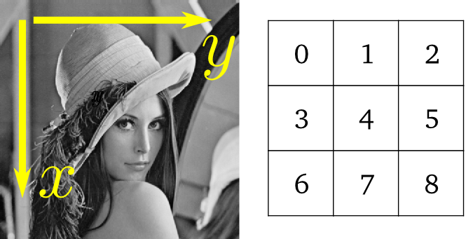
基本操作

图像是数组：使用整个numpy机理。

>>> lena = misc.lena()
>>> lena[0, 40]
166
>>> # Slicing
>>> lena[10:13, 20:23]
array([[158, 156, 157],
[157, 155, 155],
[157, 157, 158]])
>>> lena[100:120] = 255
>>>
>>> lx, ly = lena.shape
>>> X, Y = np.ogrid[0:lx, 0:ly]
>>> mask = (X - lx/2)**2 + (Y - ly/2)**2 > lx*ly/4
>>> # Masks
>>> lena[mask] = 0
>>> # Fancy indexing
>>> lena[range(400), range(400)] = 255

统计信息

>>> lena = scipy.lena()
>>> lena.mean()
124.04678344726562
>>> lena.max(), lena.min()
(245, 25)

np.histogram

几何转换

>>> lena = scipy.lena()
>>> lx, ly = lena.shape
>>> # Cropping
>>> crop_lena = lena[lx/4:-lx/4, ly/4:-ly/4]
>>> # up <-> down flip
>>> flip_ud_lena = np.flipud(lena)
>>> # rotation
>>> rotate_lena = ndimage.rotate(lena, 45)
>>> rotate_lena_noreshape = ndimage.rotate(lena, 45, reshape=False)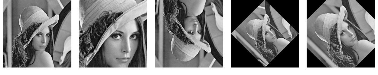

示例源码

图像滤镜

局部滤镜：用相邻像素值的函数替代当前像素的值。

相邻：方形(指定大小)，圆形，或者更多复杂的_结构元素_。

模糊/平滑

scipy.ndimage中的_高斯滤镜_：

>>> from scipy import misc
>>> from scipy import ndimage
>>> lena = misc.lena()
>>> blurred_lena = ndimage.gaussian_filter(lena, sigma=3)
>>> very_blurred = ndimage.gaussian_filter(lena, sigma=5)

均匀滤镜

>>> local_mean = ndimage.uniform_filter(lena, size=11)

示例源码

锐化

锐化模糊图像：

>>> from scipy import misc
>>> lena = misc.lena()
>>> blurred_l = ndimage.gaussian_filter(lena, 3)

通过增加拉普拉斯近似增加边缘权重：

>>> filter_blurred_l = ndimage.gaussian_filter(blurred_l, 1)
>>> alpha = 30
>>> sharpened = blurred_l + alpha * (blurred_l - filter_blurred_l)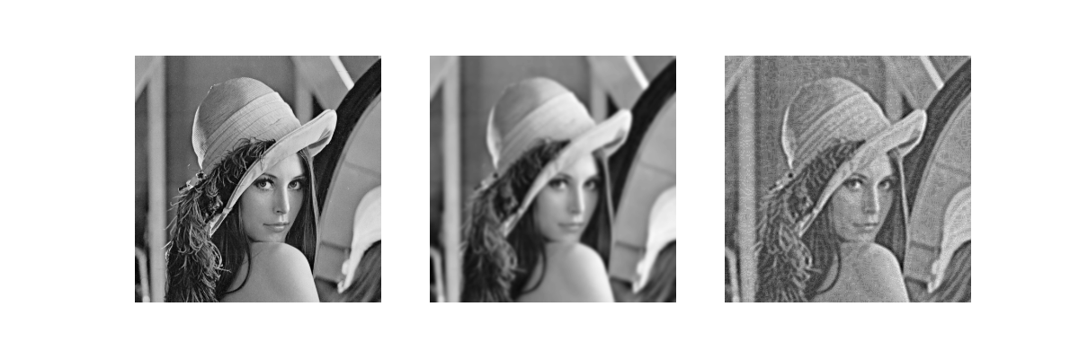

示例源码

消噪

向lena增加噪声：

>>> from scipy import misc
>>> l = misc.lena()
>>> l = l[230:310, 210:350]
>>> noisy = l + 0.4*l.std()*np.random.random(l.shape)

_高斯滤镜_平滑掉噪声……还有边缘：

>>> gauss_denoised = ndimage.gaussian_filter(noisy, 2)

大多局部线性各向同性滤镜都模糊图像(ndimage.uniform_filter)

_中值滤镜_更好地保留边缘：

>>> med_denoised = ndimage.median_filter(noisy, 3)

示例源码

中值滤镜：对直边界效果更好(低曲率)：

>>> im = np.zeros((20, 20))
>>> im[5:-5, 5:-5] = 1
>>> im = ndimage.distance_transform_bf(im)
>>> im_noise = im + 0.2*np.random.randn(*im.shape)
>>> im_med = ndimage.median_filter(im_noise, 3)

示例源码

其它排序滤波器：ndimage.maximum_filter,ndimage.percentile_filter

其它局部非线性滤波器：维纳滤波器(scipy.signal.wiener)等

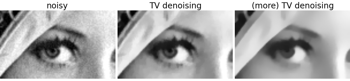
非局部滤波器

_总变差(TV)_消噪。找到新的图像让图像的总变差(正态L1梯度的积分)变得最小，当接近测量图像时：

>>> # from skimage.filter import tv_denoise
>>> from tv_denoise import tv_denoise
>>> tv_denoised = tv_denoise(noisy, weight=10)
>>> # More denoising (to the expense of fidelity to data)
>>> tv_denoised = tv_denoise(noisy, weight=50)

总变差滤镜tv_denoise可以从skimage中获得，(文档:http://scikit-image.org/docs/dev/api/skimage.filter.html#denoise-tv)，但是为了方便我们在这个教程中作为一个_单独模块_导入。

示例源码

数学形态学

参见：http://en.wikipedia.org/wiki/Mathematical_morphology

结构元素：

>>> el = ndimage.generate_binary_structure(2, 1)
>>> el
array([[False,  True, False],[ True,  True,  True],[False,  True, False]], dtype=bool)
>>> el.astype(np.int)
array([[0, 1, 0],[1, 1, 1],[0, 1, 0]])

腐蚀 = 最小化滤镜。用结构元素覆盖的像素的最小值替代一个像素值：

>>> a = np.zeros((7,7), dtype=np.int)
>>> a[1:6, 2:5] = 1
>>> a
array([[0, 0, 0, 0, 0, 0, 0],[0, 0, 1, 1, 1, 0, 0],[0, 0, 1, 1, 1, 0, 0],[0, 0, 1, 1, 1, 0, 0],[0, 0, 1, 1, 1, 0, 0],[0, 0, 1, 1, 1, 0, 0],[0, 0, 0, 0, 0, 0, 0]])
>>> ndimage.binary_erosion(a).astype(a.dtype)
array([[0, 0, 0, 0, 0, 0, 0],[0, 0, 0, 0, 0, 0, 0],[0, 0, 0, 1, 0, 0, 0],[0, 0, 0, 1, 0, 0, 0],[0, 0, 0, 1, 0, 0, 0],[0, 0, 0, 0, 0, 0, 0],[0, 0, 0, 0, 0, 0, 0]])
>>> #Erosion removes objects smaller than the structure
>>> ndimage.binary_erosion(a, structure=np.ones((5,5))).astype(a.dtype)
array([[0, 0, 0, 0, 0, 0, 0],[0, 0, 0, 0, 0, 0, 0],[0, 0, 0, 0, 0, 0, 0],[0, 0, 0, 0, 0, 0, 0],[0, 0, 0, 0, 0, 0, 0],[0, 0, 0, 0, 0, 0, 0],[0, 0, 0, 0, 0, 0, 0]])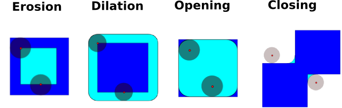

膨胀：最大化滤镜:

>>> a = np.zeros((5, 5))
>>> a[2, 2] = 1
>>> a
array([[ 0.,  0.,  0.,  0.,  0.],[ 0.,  0.,  0.,  0.,  0.],[ 0.,  0.,  1.,  0.,  0.],[ 0.,  0.,  0.,  0.,  0.],[ 0.,  0.,  0.,  0.,  0.]])
>>> ndimage.binary_dilation(a).astype(a.dtype)
array([[ 0.,  0.,  0.,  0.,  0.],[ 0.,  0.,  1.,  0.,  0.],[ 0.,  1.,  1.,  1.,  0.],[ 0.,  0.,  1.,  0.,  0.],[ 0.,  0.,  0.,  0.,  0.]])

对灰度值图像也有效：

>>> np.random.seed(2)
>>> x, y = (63*np.random.random((2, 8))).astype(np.int)
>>> im[x, y] = np.arange(8)>>> bigger_points = ndimage.grey_dilation(im, size=(5, 5), structure=np.ones((5, 5)))>>> square = np.zeros((16, 16))
>>> square[4:-4, 4:-4] = 1
>>> dist = ndimage.distance_transform_bf(square)
>>> dilate_dist = ndimage.grey_dilation(dist, size=(3, 3), \
...         structure=np.ones((3, 3)))

示例源码

开操作：腐蚀+膨胀：

应用：移除噪声

>>> square = np.zeros((32, 32))
>>> square[10:-10, 10:-10] = 1
>>> np.random.seed(2)
>>> x, y = (32*np.random.random((2, 20))).astype(np.int)
>>> square[x, y] = 1>>> open_square = ndimage.binary_opening(square)>>> eroded_square = ndimage.binary_erosion(square)
>>> reconstruction = ndimage.binary_propagation(eroded_square, mask=square)

示例源码

闭操作：膨胀+腐蚀

许多其它数学分形：击中(hit)和击不中(miss)变换，tophat等等。

特征提取

边缘检测

合成数据：

>>> im = np.zeros((256, 256))
>>> im[64:-64, 64:-64] = 1
>>>
>>> im = ndimage.rotate(im, 15, mode='constant')
>>> im = ndimage.gaussian_filter(im, 8)

使用_梯度操作(Sobel)_来找到搞强度的变化：

>>> sx = ndimage.sobel(im, axis=0, mode='constant')
>>> sy = ndimage.sobel(im, axis=1, mode='constant')
>>> sob = np.hypot(sx, sy)

示例源码

canny滤镜

Canny滤镜可以从skimage中获取(文档)，但是为了方便我们在这个教程中作为一个_单独模块_导入：

>>> #from skimage.filter import canny
>>> #or use module shipped with tutorial
>>> im += 0.1*np.random.random(im.shape)
>>> edges = canny(im, 1, 0.4, 0.2) # not enough smoothing
>>> edges = canny(im, 3, 0.3, 0.2) # better parameters

示例源码

需要调整几个参数……过度拟合的风险

分割

基于_直方图_的分割(没有空间信息)

  >>> n = 10>>> l = 256>>> im = np.zeros((l, l))>>> np.random.seed(1)>>> points = l*np.random.random((2, n**2))>>> im[(points[0]).astype(np.int), (points[1]).astype(np.int)] = 1>>> im = ndimage.gaussian_filter(im, sigma=l/(4.*n))>>> mask = (im > im.mean()).astype(np.float)>>> mask += 0.1 * im>>> img = mask + 0.2*np.random.randn(*mask.shape)>>> hist, bin_edges = np.histogram(img, bins=60)>>> bin_centers = 0.5*(bin_edges[:-1] + bin_edges[1:])>>> binary_img = img > 0.5

示例源码

自动阈值：使用高斯混合模型：

>>> mask = (im > im.mean()).astype(np.float)
>>> mask += 0.1 * im
>>> img = mask + 0.3*np.random.randn(*mask.shape)>>> from sklearn.mixture import GMM
>>> classif = GMM(n_components=2)
>>> classif.fit(img.reshape((img.size, 1)))
GMM(...)>>> classif.means_
array([[ 0.9353155 ],[-0.02966039]])
>>> np.sqrt(classif.covars_).ravel()
array([ 0.35074631,  0.28225327])
>>> classif.weights_
array([ 0.40989799,  0.59010201])
>>> threshold = np.mean(classif.means_)
>>> binary_img = img > threshold

使用数学形态学来清理结果：

>>> # Remove small white regions
>>> open_img = ndimage.binary_opening(binary_img)
>>> # Remove small black hole
>>> close_img = ndimage.binary_closing(open_img)

示例源码

练习

参看重建(reconstruction)操作(腐蚀+传播(propagation))产生比开/闭操作更好的结果：

>>> eroded_img = ndimage.binary_erosion(binary_img)
>>> reconstruct_img = ndimage.binary_propagation(eroded_img, mask=binary_img)
>>> tmp = np.logical_not(reconstruct_img)
>>> eroded_tmp = ndimage.binary_erosion(tmp)
>>> reconstruct_final = np.logical_not(ndimage.binary_propagation(eroded_tmp, mask=tmp))
>>> np.abs(mask - close_img).mean()
0.014678955078125
>>> np.abs(mask - reconstruct_final).mean()
0.0042572021484375

练习

检查首次消噪步骤(中值滤波，总变差)如何更改直方图，并且查看是否基于直方图的分割更加精准了。

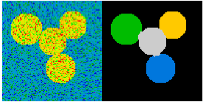
_基于图像_的分割：使用空间信息

  >>> from sklearn.feature_extraction import image>>> from sklearn.cluster import spectral_clustering>>> l = 100>>> x, y = np.indices((l, l))>>> center1 = (28, 24)>>> center2 = (40, 50)>>> center3 = (67, 58)>>> center4 = (24, 70)>>> radius1, radius2, radius3, radius4 = 16, 14, 15, 14>>> circle1 = (x - center1[0])**2 + (y - center1[1])**2 < radius1**2>>> circle2 = (x - center2[0])**2 + (y - center2[1])**2 < radius2**2>>> circle3 = (x - center3[0])**2 + (y - center3[1])**2 < radius3**2>>> circle4 = (x - center4[0])**2 + (y - center4[1])**2 < radius4**2>>> # 4 circles>>> img = circle1 + circle2 + circle3 + circle4>>> mask = img.astype(bool)>>> img = img.astype(float)>>> img += 1 + 0.2*np.random.randn(*img.shape)>>> # Convert the image into a graph with the value of the gradient on>>> # the edges.>>> graph = image.img_to_graph(img, mask=mask)>>> # Take a decreasing function of the gradient: we take it weakly>>> # dependant from the gradient the segmentation is close to a voronoi>>> graph.data = np.exp(-graph.data/graph.data.std())>>> labels = spectral_clustering(graph, k=4, mode='arpack')>>> label_im = -np.ones(mask.shape)>>> label_im[mask] = labels

测量对象属性：ndimage.measurements

合成数据：

>>> n = 10
>>> l = 256
>>> im = np.zeros((l, l))
>>> points = l*np.random.random((2, n**2))
>>> im[(points[0]).astype(np.int), (points[1]).astype(np.int)] = 1
>>> im = ndimage.gaussian_filter(im, sigma=l/(4.*n))
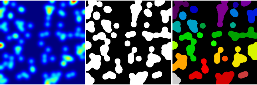
>>> mask = im > im.mean()

连接成分分析

标记连接成分：ndimage.label

  >>> label_im, nb_labels = ndimage.label(mask)>>> nb_labels # how many regions?23>>> plt.imshow(label_im)        <matplotlib.image.AxesImage object at ...>

示例源码

计算每个区域的尺寸，均值等等：

>>> sizes = ndimage.sum(mask, label_im, range(nb_labels + 1))
>>> mean_vals = ndimage.sum(im, label_im, range(1, nb_labels + 1))

计算小的连接成分：

>>> mask_size = sizes < 1000
>>> remove_pixel = mask_size[label_im]
>>> remove_pixel.shape
(256, 256)
>>> label_im[remove_pixel] = 0
>>> plt.imshow(label_im)
<matplotlib.image.AxesImage object at ...>

现在使用np.searchsorted重新分配标签：

>>> labels = np.unique(label_im)
>>> label_im = np.searchsorted(labels, label_im)

示例源码

找到关注的封闭对象区域：³

>>> slice_x, slice_y = ndimage.find_objects(label_im==4)[0]
>>> roi = im[slice_x, slice_y]
>>> plt.imshow(roi)
<matplotlib.image.AxesImage object at ...>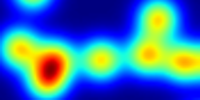

示例源码

其它空间测量：ndiamge.center_of_mass,ndimage.maximum_position等等。

可以在分割应用限制范围之外使用。

示例：块平均(block mean)：

m scipy import misc
>>> l = misc.lena()
>>> sx, sy = l.shape
>>> X, Y = np.ogrid[0:sx, 0:sy]
>>> regions = sy/6 * (X/4) + Y/6  # note that we use broadcasting
>>> block_mean = ndimage.mean(l, labels=regions, index=np.arange(1,
...     regions.max() +1))
>>> block_mean.shape = (sx/4, sy/6)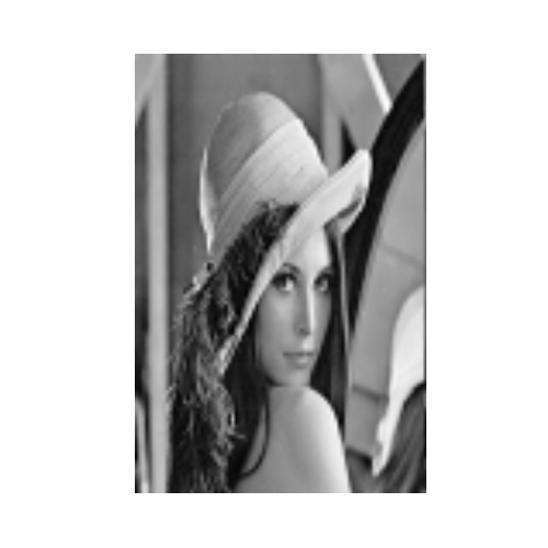

示例源码

当区域不是正则的⁴块状时，使用stride技巧更有效(示例：fake dimensions with strides)

非正则空间(Non-regular-spaced)区块：径向平均：

>>> sx, sy = l.shape
>>> X, Y = np.ogrid[0:sx, 0:sy]
>>> r = np.hypot(X - sx/2, Y - sy/2)
>>> rbin = (20* r/r.max()).astype(np.int)
>>> radial_mean = ndimage.mean(l, labels=rbin, index=np.arange(1, rbin.max() +1))

示例源码

其它测量

相关函数，傅里叶/小波谱等。

一个使用数学形态学的例子：粒度(http://en.wikipedia.org/wiki/Granulometry_%28morphology%29)

>>> def disk_structure(n):
...     struct = np.zeros((2 * n + 1, 2 * n + 1))
...     x, y = np.indices((2 * n + 1, 2 * n + 1))
...     mask = (x - n)**2 + (y - n)**2 <= n**2
...     struct[mask] = 1
...     return struct.astype(np.bool)
...
>>>
>>> def granulometry(data, sizes=None):
...     s = max(data.shape)
...     if sizes == None:
...         sizes = range(1, s/2, 2)
...     granulo = [ndimage.binary_opening(data, \
...         structure=disk_structure(n)).sum() for n in sizes]
...     return granulo
...
>>>
>>> np.random.seed(1)
>>> n = 10
>>> l = 256
>>> im = np.zeros((l, l))
>>> points = l*np.random.random((2, n**2))
>>> im[(points[0]).astype(np.int), (points[1]).astype(np.int)] = 1
>>> im = ndimage.gaussian_filter(im, sigma=l/(4.*n))
>>>
>>> mask = im > im.mean()
>>>
>>> granulo = granulometry(mask, sizes=np.arange(2, 19, 4))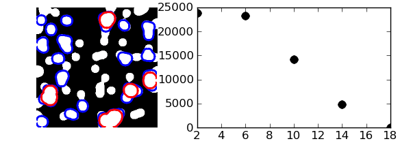

示例源码

Footnotes

占位 ↩
ValueError: can not convert int64 to uint8. ↩
根据以上操作剩下的区域选择区域，因为是随机生成可能结果不通，label_im==4未必留下来了。 ↩
正则空间 ↩