We are in a age where machines are utilizing huge data and trying to create a better world. It might range from predicting crime rates in an area using machine learning to conversing with humans using natural language processing. In this blog article, I am going to take you through a real-world data science problem which I have picked from UCI machine learning repository and will demonstrate my way of solving it. This case study solves everything right from scratch. Starting from data analysis and taking you through feature engineering and at last model building with both machine learning and deep learning models.

我们正处于一个机器正在利用海量数据并试图创造一个更美好世界的时代。 它的范围可能从使用机器学习预测某个地区的犯罪率到使用自然语言处理与人交谈。 在这篇博客文章中，我将带您解决一个现实世界中的数据科学问题，该问题是我从UCI机器学习存储库中挑选的，并展示了解决该问题的方法。 本案例研究从头解决了所有问题。 从数据分析开始，带您进行功能工程，最后使用机器学习和深度学习模型构建模型。

Note: Full code and data files are available on my Git-hub repo here.

注意 ：完整的代码和数据文件可在此处的Git-hub存储库中找到。

Problem Statement

问题陈述

It can be hard to know whether a patient will be readmitted to the hospital, it might mean the patient didn’t get the best treatment on the last occasion he/she was admitted or the patient might be diagnosed wrongly and treated for a different disease altogether. The patient when seen at first can’t be predicted whether he/she will be readmitted or not but lab reports and the details of type of patient can be very useful in predicting whether the patient might be readmitted within 30 days. The main objective of this case study is to check whether the patient with diabetes will be readmitted to the hospital within 30 days.

很难知道患者是否会再次入院，这可能意味着该患者在上次入院时未获得最佳治疗，或者可能被错误诊断并接受其他疾病的治疗共。 初诊时无法预测患者是否会再次入院，但是实验室报告和患者类型的详细信息对于预测患者是否会在30天内再次入院非常有用。 该案例研究的主要目的是检查糖尿病患者是否会在30天内再次入院。

指数： (Index:)

• Step-1: Mapping the real world problem to a Machine Learning Problem.

  步骤1：将现实世界问题映射到机器学习问题。

• Step-2: Exploratory Data Analysis by performing uni variate, bi variate and multi variate analysis on the data.

  步骤2：通过对数据执行单变量，双变量和多变量分析来探索数据。

• Step-3: Feature engineering by adding new features and selecting important features from the data.

  步骤3：通过添加新功能并从数据中选择重要功能来进行功能工程。

• Step-4: Creating machine learning and deep learning models to predict hospital readmission.

  步骤4：创建机器学习和深度学习模型以预测住院率。

步骤1：将现实世界问题映射到机器学习问题 (Step 1: Mapping the real world problem to a Machine Learning Problem)

机器学习问题的类型： (Type of Machine Learning Problem:)

For the given patient we must predict whether the patient will be readmitted within 30 days or not given patient details including the diagnosis and medications the patient has taken.

对于给定的患者，我们必须预测患者是否会在30天内重新入院，或者是否没有给出患者的详细信息，包括患者的诊断和用药。

The given problem is a classification problem as it will return whether the patient will be readmitted within 30 days or not.

给定的问题是分类问题，因为它将返回是否在30天内重新接纳患者。

Error metric : F1 score and AUC(Area under curve) score.

误差度量： F1得分和AUC(曲线下面积)得分。

Data

数据

Data overview:

数据概述：

Get the data from : https://archive.ics.uci.edu/ml/datasets/Diabetes+130-US+hospitals+for+years+1999-2008#

从以下网址获取数据： https : //archive.ics.uci.edu/ml/datasets/Diabetes+130-US+hospitals+for+years+1999-2008#

The dataset represents 10 years (1999–2008) of clinical care at 130 US hospitals and integrated delivery networks. It includes over 50 features representing patient and hospital outcomes. Information was extracted from the database for encounters that satisfied the following criteria.

该数据集代表了美国130家医院和综合交付网络的10年(1999-2008年)临床护理。 它包括代表患者和医院结果的50多种功能。 从数据库中提取满足以下条件的遭遇信息。

(1) It is an inpatient encounter (a hospital admission).

(1)这是住院期间(住院)。

(2) It is a diabetic encounter, that is, one during which any kind of diabetes was entered to the system as a diagnosis.

(2)这是一种糖尿病的遭遇，即在此期间将任何类型的糖尿病输入系统以进行诊断。

(3) The length of stay was at least 1 day and at most 14 days.

(3)住院时间至少1天，最多14天。

(4) Laboratory tests were performed during the encounter.

(4)在相遇期间进行了实验室测试。

(5) Medications were administered during the encounter.

(5)在相遇期间服用药物。

The data contains such attributes as patient number, race, gender, age, admission type, time in hospital, medical specialty of admitting physician, number of lab test performed, HbA1c test result, diagnosis, number of medication, diabetic medications, number of outpatient, inpatient, and emergency visits in the year before the hospitalization, etc.

数据包含以下属性：患者编号，种族，性别，年龄，入院类型，住院时间，主治医师的医学专业，进行化验的次数，HbA1c测试结果，诊断，用药次数，糖尿病用药，门诊人数住院前一年的住院，住院和急诊就诊等

We will be looking into each of the 50 features in detail when we perform exploratory data analysis.

在进行探索性数据分析时，我们将详细研究这50个功能。

Target variable: Readmitted

目标变量：允许

We will build various machine learning and deep learning models and see which provides the best result. Now let us start with exploratory data analysis

我们将构建各种机器学习和深度学习模型，并查看哪种模型可以提供最佳结果。 现在让我们开始探索性数据分析

第2步：探索性数据分析 (Step 2:Exploratory Data Analysis)

The very first step in solving any case study in data science is to properly look and analyze the data. It helps to give valuable insights and information. Statistical tools has a big role in proper visualization of the data. ML engineers spend maximum part of solving a problem by analyzing the data they have and this step is considered as an important step as it helps us to understand the data precisely. Proper EDA gives interesting features of your data which in turn influences our data preprocessing and model selection criterion as well.

解决数据科学中任何案例研究的第一步就是正确地查找和分析数据。 它有助于提供有价值的见解和信息。 统计工具在适当地可视化数据方面起着重要作用。 机器学习工程师通过分析他们拥有的数据来最大程度地解决问题，这一步骤被认为是重要的一步，因为它有助于我们准确地理解数据。 适当的EDA可以为您的数据提供有趣的功能，进而影响我们的数据预处理和模型选择标准。

加载数据： (Loading the data:)

To load the data, we only need the diabetic_data.csv file. We will load this into a pandas dataframe.

要加载数据，我们只需要diabetic_data.csv文件。 我们将其加载到pandas数据框中。

There are a total of 101766 patient records with 50 features for each record. The first 5 patient records can be seen above.

共有101766个患者记录，每个记录具有50个功能。 前5个患者记录可以在上方看到。

检查多次住院访问： (Checking multiple inpatient visits:)

The data contains multiple inpatient visits for some patients, I have considered only the first encounter for each patient to determine whether or not they were readmitted within 30days. So the duplicate values are removed.

数据包含某些患者的多次住院就诊，我仅考虑了每位患者的初次会诊以确定他们是否在30天内再次入院。 因此，删除了重复的值。

#creating new column duplicate which contains whether the row is duplicated or not. It is boolean.
data['duplicate'] = data['patient_nbr'].duplicated()
#only those rows which are not duplicated are kept in the dataset.
data = data[data['duplicate'] == False]#the duplicate column is dropped.
data = data.drop(['duplicate'], axis = 1)

Removing patients who are dead or in hospice:

转移死亡或临终关怀的患者：

The dataset also contains patients who are dead or in hospice. In the IDs_mapping.csv provided in https://www.hindawi.com/journals/bmri/2014/781670/#supplementary-materials we can see that 11,13,14,19,20,21 are related to death or hospice. We should remove these samples from the data since they cannot be readmitted.

该数据集还包含已死亡或临终关怀的患者。 在https://www.hindawi.com/journals/bmri/2014/781670/#supplementary-materials中提供的IDs_mapping.csv中，我们可以看到11,13,14,19,20,21与死亡或临终关怀有关。 我们应该从数据中删除这些样本，因为它们无法重新读取。

#removing the patients who are dead or in hospice.
data = data.loc[~data['discharge_disposition_id'].isin([11,13,14,19,20,21])]

We are left with 69,973 patients who are not dead and not in hospice.

我们剩下69,973名尚未死亡且没有临终关怀的患者。

检查数据集中的空值： (Checking for null values in the data set:)

The nan values are represented as ‘?’ in the dataset. We will replace ? with nan and then check the total nan values in the dataset.

nan值表示为“？” 在数据集中。 我们会更换吗？ 使用nan，然后检查数据集中的总nan值。

We will be checking the percentage of null values in each feature,

我们将检查每个功能中空值的百分比，

(data.isna().sum()/len(data))*100

7 features contain null values.

7个要素包含空值。

We can observe that weight has the highest null values at 96%. Medical specialty and payer code have 48% and 43% null values respectively. The weight feature can be dropped since there is very high percentage of null values.

我们可以看到，权重值在96％处具有最高的空值。 医学专业和付款人代码的空值分别为48％和43％。 由于存在很高百分比的空值，因此可以删除权重功能。

The payer code and medical specialty column missing values can be found using imputation techniques since more than 50% data is available in both cases. We will be dealing with this features afterwards.

可以使用归因技术找到付款人代码和医疗专业栏的缺失值，因为在两种情况下都可获得50％以上的数据。 之后，我们将处理此功能。

单变量分析： (Uni variate Analysis:)

Race:

种族：

The race column consists of Caucasian,AfricanAmerican, Hispanic, Asian and other as categories. It consists of 2.7% NaN values

种族栏包括高加索人，非裔美国人，西班牙裔，亚洲人和其他类别。 它由2.7％的NaN值组成

We can see that the patients are dominated by Caucasian people, followed by African American’s and Asian’s are least in number. The nan values are filled with mode of race feature.

我们可以看到，患者以白人为主，其次是非洲裔美国人和亚裔。 nan值填充了竞赛模式功能。

Gender:

性别：

The gender column tells us whether the patient is male or female.

性别栏告诉我们患者是男性还是女性。

3 values are unknown. We can either fill these values or drop the rows. Dropping the rows would be better since the data is also considered as invalid/Unknown in case of gender.

3个值未知。 我们可以填充这些值或删除行。 删除行会更好，因为在性别情况下，数据也被视为无效/未知。

• The female count is more than male count but the difference is small.女性人数多于男性人数，但差异很小。
• I have encoded the label of male to 1 and female to 0.我已经将男性标签编码为1，女性标签编码为0。

Age:

年龄：

• As expected, the patients with age less than 40 years are less in number when compared to patients with age greater than 40 years.不出所料，年龄小于40岁的患者与年龄大于40岁的患者相比数量较少。
• The number of patients are highest in the age group of 70–80 years.70-80岁年龄段的患者人数最多。

I will be grouping the age feature into 3 categories as mentioned in the research paper (https://www.hindawi.com/journals/bmri/2014/781670/).

我将把年龄特征分为研究论文( https://www.hindawi.com/journals/bmri/2014/781670/ )中提到的3类。

#custom encoding age
data.loc[data['age'] == '[0-10)', ['age']] = 0
data.loc[data['age'] == '[10-20)', ['age']] = 0
data.loc[data['age'] == '[20-30)', ['age']] = 0
data.loc[data['age'] == '[30-40)', ['age']] = 1
data.loc[data['age'] == '[40-50)', ['age']] = 1
data.loc[data['age'] == '[50-60)', ['age']] = 1
data.loc[data['age'] == '[60-70)', ['age']] = 2
data.loc[data['age'] == '[70-80)', ['age']] = 2
data.loc[data['age'] == '[80-90)', ['age']] = 2
data.loc[data['age'] == '[90-100)', ['age']] = 2

The plot after grouping age looks like this,

分组年龄后的图看起来像这样，

Admission_type_id： (Admission_type_id:)

The mappings can be obtained from mappings given in uiuc,

可以从uiuc中给定的映射获得映射，

In Admission_type_id most of the patients are admitted with id emergency, followed by Elective. Some of the patients admission type id is not available. Null and Not mapped categories are also present.

在Admission_type_id中，大多数患者因急诊入院，其次是选修科。 某些患者的入院类型ID不可用。 空和未映射类别也存在。

Discharge_disposition_id： (Discharge_disposition_id:)

The discharge disposition id consists of 29 categories of id’s.

排放处置ID由29个ID类别组成。

• The discharge_disposition_id column is divided into 21 different categories which is then changed to 8 categories after careful observationsdischarge_disposition_id列分为21个不同的类别，经过仔细观察，然后将其更改为8个类别

• We can observe that most of the patients are discharged to home.我们可以观察到，大多数患者已出院回家。
• The patients who have passed away or in hospice are not present since we have already removed those rows from the data.因为我们已经从数据中删除了那些行，所以没有人去世或临终关怀。

mission_source_id： (admission_source_id:)

• admission_source_id mappings are given in the ids_mappings.csv present in UCI.UCI中存在的ids_mappings.csv中提供了admission_source_id映射。
• The categories were changed from 17 to 8.类别从17更改为8。

• We can observe that most of the patients admission source is emergency room, followed by referrals.我们可以观察到，大多数患者的入院来源是急诊室，其次是转诊。

医院时间： (Time_in_hospital:)

• The time in hospital column categorizes the patients stay ranging from 1 day to 14 days.“住院时间”列将患者停留的时间分类为1天至14天。

• The patients on average stay 4 days and most patients stay 3–4 days.患者平均住院4天，大多数患者住院3-4天。
• The patients rarely stay more than 12 days.患者很少停留超过12天。
• We can observe a positive skew in the plot.我们可以在图中观察到正偏斜。

num_lab_procedures： (num_lab_procedures:)

Refers to number of lab tests performed during the encounter.

指在遭遇期间执行的实验室测试的数量。

• We can observe that on average 43 lab procedures are done during a patient encounter.我们可以观察到，在遇到患者期间平均执行了43个实验室程序。
• A spike is also found near 0–2 procedures which suggest less number of lab tests were done on some patients.在0–2程序附近也发现一个峰值，这表明对某些患者进行的实验室检查次数减少。

Num_procedures： (Num_procedures:)

Refers to number of procedures (other than lab tests) performed during the encounter

指相遇期间执行的步骤数(实验室测试除外)

Most of the patients do not perform tests other than lab tests. Positive skew is observed.

除实验室测试外，大多数患者不执行其他测试。 观察到正偏斜。

药物编号： (Num_medications:)

Refers to number of distinct generic names administered during the encounter

指遇到期间管理的不同通用名称的数量

• Most of the patients are provided 16 medications on average.大多数患者平均获得16种药物治疗。
• Only 7 patients are given more than 70 medications.仅7例患者接受了超过70种药物治疗。
• The plot has positive skewness and resembles normal distribution.该图具有正偏度并且类似于正态分布。

门诊人数： (Number_outpatient:)

Refers to number of outpatient visits of the patient in the year preceding the encounter

指患者在遭遇前一年的门诊次数

• We can observe that most of the patients do not have any outpatient visits.我们可以观察到，大多数患者没有任何门诊就诊。
• Very less patients have more than 15 outpatient visits很少有超过15位门诊病人

紧急电话： (Number_emergency:)

• It is similar to number_outpatient distplot.它类似于number_outpatient distplot。
• We can observe that most of the patients do not have any emergency visits.我们可以观察到，大多数患者没有任何急诊就诊。

住院人数： (Number_inpatient:)

• We can observe that most of the patients do not have any inpatient visits.我们可以观察到，大多数患者没有任何住院访问。
• It is similar to other visit figures seen.这与其他访问数据相似。
• We can create a new feature ‘visits’ which will be some of inpatient, outpatient and emergency visits since all three are distributed in similar ways.我们可以创建一个新的“访问”功能，其中包括住院，门诊和急诊就诊，因为这三种方式均以相似的方式分配。

诊断： (Diagnosis:)

All three diagnosis features contain code which are categorized into one of the 9 groups. The groups are given in the research paper.We can categorize these codes into the 9 categories and use them as diagnosis of diseases which come under these 9 categories. This idea has been taken from the research paper.

所有这三个诊断功能都包含归类为9组之一的代码。 研究组中给出了这些组。我们可以将这些代码分为9类，并将它们用作这9类中的疾病诊断。 这个想法来自研究论文。

The new categories are analyzed,

分析了新类别，

• In the second and third diagnosis we can observe that more number of patients are getting diagnosed with 4 which is diabetes mellitus.在第二和第三次诊断中，我们可以观察到越来越多的患者被诊断出患有4种糖尿病。
• Most of the patients are diagnosed with respiratory and other disease types.大多数患者被诊断出患有呼吸系统疾病和其他疾病。
• The nan category also increase with diagnosis number. It is represented as -1 in the feature.nan类别也随着诊断次数的增加而增加。 在要素中以-1表示。

编号诊断 (Number_diagnoses)

Refers to the number of diagnoses entered to the system

指输入到系统的诊断数

• Most patients have undergone 9 diagnoses.大多数患者已进行了9次诊断。
• More than 9 diagnoses is rare.很少有9个以上的诊断。

Max_glu_serum (Max_glu_serum)

Indicates the range of the result or if the test was not taken. Values: “>200,” “>300,”“normal,” and “none” if not measured

指示结果范围或未进行测试。 值：“> 200”，“> 300”，“正常”和“无”(如果未测量)

• Most of the patients dont undergo this test.大多数病人不接受这项检查。
• Out of the people who undergo this test about half of the patients result are normal, the other half patients result are either in category >200 or >300.在接受该测试的人中，约一半的患者结果是正常的，另一半患者的结果属于> 200或> 300。
• Ordinal encoding is done since max_glu_serum above certain values indicate the value is abnormal for the patient and hence are more important in predicting the re admittance.由于max_glu_serum高于某些值表示该值对于患者而言异常，因此进行了序数编码，因此在预测再吸收率方面更重要。

A1结果 (A1Cresult)

Indicates the range of the result or if the test was not taken. Values: “>8” if the result was greater than 8%, “>7” if the result was greater than 7% but less than 8%, “normal” if the result was less than 7%, and “none” if not measured.

指示结果范围或未进行测试。 值：如果结果大于8％，则为“> 8”；如果结果大于7％但小于8％，则为“> 7”；如果结果小于7％，则为“正常”；如果结果大于7％，则为“无”。没有测量。

• Most of the patients don't undergo this test.大多数病人不接受这项检查。
• Out of the people who undergo this test nearly half of the patients result are >8, the other half patients result are either in >7 or normal category.在接受这项测试的人中，近一半的患者结果> 8，另一半的患者结果为> 7或正常类别。
• Ordinal encoding is done since A1Cresult above certain values indicate the value is abnormal for the patient and hence are more important由于A1Cresult高于某些值表示该值对于患者而言异常，因此进行了序数编码，因此更重要

药物治疗 (Medications)

Values: “up” if the dosage was increased during the encounter, “down” if the dosage was decreased, “steady” if the dosage did not change, and “no” if the drug was not prescribed.

值：如果在相遇期间增加剂量，则为“向上”；如果减少剂量，则为“向下”；如果剂量不变，则为“稳定”；如果未开药，则为“否”。

There are a total of 23 medications and values for each medications is given. When analyzed, it was found that 3 medications were not prescribed for any patient. These 3 features don't help to classify whether the patient readmitted within 30 days as all the values are same. So these features are dropped from the dataset.

一共有23种药物，每种药物的值均已给出。 经过分析，发现没有为任何患者开3种药物。 这三个功能无法对患者是否在30天内重新入院进行分类，因为所有值都相同。 因此，这些特征已从数据集中删除。

The medications can be merged into a single feature and the number of medications a patients has taken can be calculated.The custom encoding of medication was done with any change in dosage resulting in 2, steady given as 1 and if the medication was not required then it is represented as 0.

可以将这些药物合并为一个特征，并可以计算出患者服用的药物数量。对药物的自定义编码是在剂量发生任何变化的情况下进行的，结果为2，稳定为1，如果不需要药物，则它表示为0。

更改： (Change:)

Indicates if there was a change in diabetic medications (either dosage or generic name). Values: “change” and “no change”

指示糖尿病药物(剂量或通用名称)是否发生变化。 值：“更改”和“不变”

• More than 50% of patients did not get any changes in the medicine, the other patients changed medicines.超过50％的患者没有改变药物，其他患者改变了药物。
• The change feature was encoded with 0 representing no change and 1 representing change in medication.更改特征编码为0表示无更改，而1表示药物更改。

糖尿病 (DiabetesMed:)

Indicates if there was any diabetic medication prescribed. Values: “yes” and “no”.

指示是否有任何糖尿病药物处方。 值：“是”和“否”。

• Most of the patients were prescribed diabetes medication.大多数患者都开了糖尿病药物。
• The diabetesMed feature was encoded with 0 representing not prescribed and 1 representing medicine prescribed.糖尿病特征编码为0表示未开处方，1表示开药。

重新提交： (Readmitted:)

This the the variable which we must predict.

这是我们必须预测的变量。

It refers to days to inpatient readmission. Values: “< 30” if the patient was readmitted in less than 30 days, “>30” if the patient was readmitted in more than 30 days, and “No” for no record of readmission.

指住院再入院的天数。 值：如果在不到30天的时间内再次入院，则为“ <30”；如果在超过30天的时间内再次入院，则为“> 30”，对于没有再入院记录，则为“否”。

• We must predict whether the patient is readmitted within 30 days.我们必须预测患者是否会在30天内再次入院。
• From the graph we can observe that less number of people are readmitted within 30 days and most of the people are either not readmitted or are readmitted after 30 days.从图中可以看出，在30天内重新接纳的人数减少了，大多数人在30天内未重新接纳或重新接纳。
• oversampling/ under sampling techniques will be required to make the data balanced.为了使数据平衡，将需要过采样/欠采样技术。

付款人代码： (Payer_code:)

As mentioned in the section before, the payer_code feature consists of 43% of null values. These null values can be filled by values predicted from model based imputation techniques. Here i have used KNN and randomforest models for imputation.

如前一节所述，payer_code功能由43％的空值组成。 这些空值可以由基于模型的插补技术预测的值填充。 在这里，我使用了KNN和randomforest模型进行插补。

There are a total of 17 types of payer codes. The payer code feature is encoded and separated from other columns. The other features of the payer code for which the values are not null are used as the training dataset and a model is fit on this data. The null values in the payer code are predicted using the model. KNN and randomforest models were used on the data and after hyperparameter tuning it was found that randomforest model perform better on predicting the null values when compared to KNN.

共有17种类型的付款人代码。 付款人代码功能已编码并与其他列分开。 值不为空的付款人代码的其他功能用作训练数据集，并且模型适合该数据。 使用该模型可以预测付款人代码中的空值。 在数据上使用了KNN和randomforest模型，经过超参数调整后，发现与KNN相比，randomforest模型在预测空值方面表现更好。

• We can observe that after imputation, the number of patients for whom the payment was done by medicare has increased drastically as expected. It was the most populated column before imputation also.我们可以观察到，在估算之后，通过医疗保险为患者付款的患者数量急剧增加。 这也是插补前人口最多的一列。
• Other categories have seen 10% increase in number at most after imputation.估算后，其他类别的数量最多增加10％。
• The plot strikes as a case of pareto distribution.该情节是作为pareto分配的情况罢工的。

medical_specialty： (medical_specialty:)

Integer identifier of a specialty of the admitting physician, corresponding to 84 distinct values, for example, cardiology, internal medicine, family\general practice, and surgeon

主治医师专科的整数标识符，对应于84个不同的值，例如心脏病学，内科医学，家庭\普通执业和外科医生

The medical specialty feature consists of 48% of null values. These null values can be filled by values predicted from model based imputation techniques. Here i have used KNN and randomforest models for imputation. There are 70 different medical specialty categories.

医学专业功能包含48％的空值。 这些空值可以由基于模型的插补技术预测的值填充。 在这里，我使用了KNN和randomforest模型进行插补。 有70个不同的医学专业类别。

The medical specialty feature is encoded using scikit-learn’s label encoder. Only the values which are not null are encoded and the features except medical specialty are used for predicting medical specialty. The null values in the medical specialty are predicted using the model fit on the other features. KNN and randomforest models were used on the data and after hyperparameter tuning it was found that randomforest model perform better on predicting the null values when compared to KNN. The encoded features are decoded using inverse transform of scikit-learn’s label encoder.

使用scikit-learn的标签编码器对医学专业功能进行编码。 只有非零值会被编码，医学专业以外的功能将用于预测医学专业。 使用在其他特征上拟合的模型来预测医学专业中的空值。 在数据上使用了KNN和randomforest模型，经过超参数调整后，发现与KNN相比，randomforest模型在预测空值方面表现更好。 编码的特征使用scikit-learn的标签编码器的逆变换进行解码。

The plots contain many categories and cannot be shown, please check the notebook mentioned if interested.

这些图包含许多类别，无法显示，如果感兴趣，请检查提到的笔记本。

• The InternalMedicine category has multiplied 3 fold after filling the missing values through imputation.通过插补填补缺失值后，InternalMedicine类别增加了3倍。
• Other categories have nearly doubled after imputation.估算后，其他类别几乎翻了一番。
• The InternalMedicine category dominates followed by family/general, cardiology and emergency/Trauma.内部医学类别占主导地位，其次是家庭/普通科，心脏病科和急诊/创伤科。

单变量分析的结论： (Conclusion of Univariate analysis:)

• The outpatient, inpatient and emergency visits can be merged into a new feature visits.门诊，住院和急诊就诊可以合并为新的功能就诊。
• Three features from medications are removed since they do not provide any information which might help to predict readmission of patients.从药物中删除了三个特征，因为它们没有提供任何有助于预测患者再入院的信息。
• The medications can be merged into a single feature and the number of medications a patients has taken can be calculated.可以将药物合并为一个特征，并可以计算患者服用的药物数量。
• The diagnosis features have been changed from icd9 codes to 10 different categories. The plots indicate that the diagnosis of diabetes mellitus increase as the number of diagnosis increase.诊断功能已从icd9代码更改为10个不同的类别。 该图表明糖尿病的诊断随着诊断次数的增加而增加。
• Model based imputation was applied on the features with missing values.基于模型的归因应用于具有缺失值的特征。
• The categorical labels can be one hot encoded to convert categorical labels to numerical data.类别标签可以是一种热编码的，用于将类别标签转换为数值数据。
• The data is highly unbalanced with only 9% of patients being readmitted within 30 days. over sampling must be done.数据高度不平衡，只有9％的患者在30天内重新入院。 必须进行过度采样。

双变量和多变量分析： (Bi variate and multivariate analysis:)

Only plots which had some observations have been plotted, other plots which didn’t any useful information have been discarded.

仅绘制了具有某些观察结果的地块，其他没有任何有用信息的地块则被丢弃。

Age:

年龄：

• Most of the readmitted patients are from age 60–100 which is category 2 in this case.大部分重新入院的患者年龄在60-100岁之间，在这种情况下属于第二类。
• The readmission increases with age.再入院人数随年龄增长而增加。
• the patients in age category 1 had primary diagnosis of 0 and 4 more in number.年龄类别1的患者的主要诊断为0和4。
• The patients in age category 2 had primary diagnosis of 0&1 more in number.初次诊断为2岁的患者人数增加了0-1。
• The patients in age category 3 had primary diagnosis of 2 more in number followed by diagnosis 2.年龄类别3的患者初步诊断为多2例，其次为诊断2。
• The patients in category 3 stayed in hospital for more time and than category 1 and 2.3类患者比1类和2类患者住院时间更长。
• The readmitted patients are diagnosed with category 0,1 and 4 diseases.重新入院的患者被诊断患有0、1和4类疾病。

Race :

种族：

• Asian, other race and Hispanic patients show similarity when compared among most of the features.在大多数特征之间进行比较时，亚裔，其他种族和西班牙裔患者表现出相似性。
• The mean of African American patients time in hospital is more compared to other race patients.与其他种族患者相比，非裔美国人患者住院时间的平均值更高。
• African American patients are admitted under category 1 which is not the case in other patients who are admitted under category 2.非裔美国人患者属于第1类，而其他非患者则属于第2类。
• Readmitted patients have stayed more than non-readmitted patients when time in hospital is taken into consideration except asian patients.考虑到住院时间，再住院患者比未再住院患者住院的时间要多，亚洲患者除外。
• other race patients who have readmitted have mean admission id as 1 when compared to non-readmitted other race patients who have mean admission id as 2.与重新入院的其他种族患者的平均入院ID为2相比，其他已入院的种族患者的平均入院ID为1。

Gender:

性别：

• Females spend more time in hospital when compared to male patients.与男性患者相比，女性在医院花费的时间更多。
• In case of readmitted patients, male readmitted patients paitents tend to spend more time in hospital when compared to male non-readmitted patients.对于再入院患者，男性再入院患者与男性未入院患者相比倾向于在医院花费更多的时间。
• most of the male readmitted patients were diagnosed as category 1 whereas most of the male non-readmitted patients were diagnosed as category 2.大部分男性重新入院患者被诊断为1类，而大多数男性未重新入院患者被诊断为2类。
• Most Males have admission id as 2 whereas most females have admission id as 1.大多数男性的入场ID为2，而大多数女性的入场ID为1。

Admission type id:

入场类型ID：

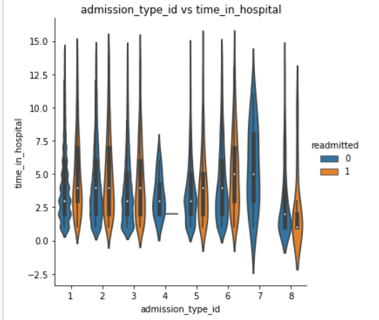
• The patients who were admitted under id 7 spent more time in hospital than other admission id patients.根据ID 7入院的患者比其他ID入院的患者住院时间更长。
• The patients who were admitted under id 8 spent least time in hospital than other admission id patients.与其他入院id患者相比，在id 8下入院的患者住院时间最少。
• For admission id 7 patients payment was most done through code SI.对于ID为7的入院患者，付款大部分通过代码SI完成。
• Less patients were readmitted who were having admission id as either 4 or 7.再次入院的ID为4或7的患者较少。
• In category 1,3,5 and 6 readmitted patients spent more time in hospital whereas in category 8 readmitted patients spent less time in hospital when compared to non-readmitted patients.在第1、3、5和6类中，再入院的患者在医院的时间更长，而在第8类中，再入院的患者与未入院的患者相比，住院时间更少。
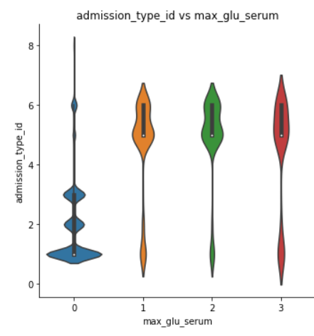
• Most max_glu_serum test were done when patients were admitted under category 5,6 and 7. For patients under category 1,2,3 less max_glu_serum tests were done.大多数max_glu_serum测试是在患者进入5,6和7类时完成的。对于1,2,3类患者，max_glu_serum测试较少。

discharge_disposition_id： (discharge_disposition_id:)

• Readmitted patients with discharge id 3 spent more time in hospital when compared to non-readmitted patients with id 3.与3的非再次入院患者相比，3的再次入院患者在医院花费的时间更长。
• Most of the readmitted patients with discharge id 3 spent had been diagnosed of category 2 disease when compared to non-readmitted patients with id 3 who were diagnosed of category 1.与没有被诊断为1类的ID为3的非再次入院患者相比，大多数已获得ID 3的再次入院患者已被诊断为2类疾病。

Plotting Correlation matrix:

绘制相关矩阵：

A correlation matrix is basically a covariance matrix that is a very good technique of multivariate exploration.

相关矩阵基本上是协方差矩阵，是一种很好的多元探索技术。

• From the above matrix we can observe that features like num_medications,number_diagnoses, num_lab_procedures tend to have positive correlation with time in hospital.从上面的矩阵中，我们可以观察到诸如num_medications，number_diagnoses，num_lab_procedures之类的特征往往与医院的时间呈正相关。
• Diagnosis features show very less correlation with other features.诊断功能与其他功能的相关性非常低。
• Readmitted also shows low correlation with other features indication linear relationship is not present with the features.再读也显示与其他特征的相关性低，表明特征不存在线性关系。

使用VIF值检查多重共线性： (Checking Multi-collinearity with VIF values:)

Variance Inflation Factor or VIF, gives a basic quantitative idea about how much the feature variables are correlated with each other.

方差通货膨胀系数或VIF给出了有关特征变量相互关联的基本定量概念。

On checking the VIF for our features, the number_diagnoses has vif value of 15.7 and age has vif value of 10, which are more than 10. After dropping number_diagnoses feature, the vif value for all features remained below 10.

在检查功能的VIF时，number_diagnoses的vif值为15.7，age的vif值为10，大于10。删除number_diagnoses功能后，所有功能的vif值均保持在10以下。

二元和多元分析的结论： (Conclusion of bivariate and multivariate analysis:)

• Asian, other race and Hispanic patients show similarity when compared among most of the features.在大多数特征之间进行比较时，亚裔，其他种族和西班牙裔患者表现出相似性。
• Readmitted patients have stayed more than non-readmitted patients on average when time in hospital is taken into consideration except asian patients.考虑到住院时间，除亚洲患者外，再入院患者的平均住院时间要多于未入院患者。
• Females spend more time in hospital when compared to male patients on average.与男性患者相比，女性平均在医院花费的时间更多。
• Most Male patients have admission id as 2 whereas most female patients have admission id as 1.大多数男性患者的入院ID为2，而大多数女性患者的入院ID为1。
• Most max_glu_serum test were done when patients were admitted under category 5,6 and 7. For patients under category 1,2,3 less max_glu_serum tests were done.大多数max_glu_serum测试是在患者进入5,6和7类时完成的。对于1,2,3类患者，max_glu_serum测试较少。
• Readmission has less correaltion with other features.重新录入与其他功能的关联度较低。
• Time in hospital has good correlation with other variables.住院时间与其他变量具有良好的相关性。
• number_diagnosis feature has high VIF value and hence it is removed. After its removal the VIF value of other features remains in the range of 0–10.number_diagnosis功能部件的VIF值较高，因此已被删除。 删除后，其他特征的VIF值仍在0-10范围内。

步骤3：功能工程： (Step 3: Feature engineering:)

访问功能： (visits feature:)

As seen in uni variate analysis the inpatient visits, outpatient visits and emergency visits can be combined into a single feature called visits. Since many of the patients didn’t get visited by anyone, we can make the visit feature binary meaning the feature can be whether the patient got visits or not. This can be done by replacing the patients who got visits by 1.

从单变量分析中可以看出，住院访问，门诊访问和紧急访问可以合并为一个称为访问的功能。 由于许多患者都没有被任何人探视，因此我们可以将探视功能设为二进制，这意味着该功能可以取决于患者是否有探视。 这可以通过将拜访的患者替换为1来完成。

The inpatient, outpatient and emergency visits feature are dropped.

住院，门诊和急诊功能已删除。

每个患者特征使用的稳定药物数量和增加/减少的药物 (number of steady medicines and increase/decrease of medicine given to each patient feature)

Two new features are derived from the 23 medication features present in the dataset. The first feature is ‘steady’ which tells us how many number of medications the patient is taking steadily. The second feature is up/down which tells us how many number of medications have been increased or decreased or changed in dosage for the patient.

从数据集中存在的23种用药特征中衍生出两个新特征。 第一个特征是“稳定”，它告诉我们患者稳定服用了多少种药物。 第二个功能是向上/向下，它告诉我们为患者增加或减少或更改了剂量的药物数量。

功能选择 (Feature Selection)

Before applying any machine learning model, our data must be fed to models in proper format. In our problem, most of the data in the columns is of categorical nature. Hence, they have to be converted to numerical format to extract relevant information. Though there are many ways to handle categorical data, one of the commonest way is to do One-Hot Encoding. Here i had used get_dummies of pandas to achieve one hot encoded features.

在应用任何机器学习模型之前，我们的数据必须以正确的格式输入模型。 在我们的问题中，列中的大多数数据都是分类性质的。 因此，必须将它们转换为数字格式以提取相关信息。 尽管有许多处理分类数据的方法，但最常见的方法之一是进行单热编码。 在这里，我使用了熊猫的get_dummies实现了一种热编码功能。

We will split our data set into train and test. Since the data is imbalanced we will be applying SMOTE to achieve balanced dataset by oversampling.We will be oversampling only the train data and not the test data. We shall fit on the entire train data and use test part for prediction purpose. Also, we shall evaluate which model performs the best on test data based on our evaluation metric AUC and f1 score.

我们将数据集分为训练和测试。 由于数据不平衡，我们将使用SMOTE通过过采样来获得平衡的数据集，我们将仅对火车数据而不对测试数据进行过采样。 我们将拟合整个火车数据，并使用测试部分进行预测。 同样，我们将根据我们的评估指标AUC和f1分数评估哪种模型在测试数据上表现最佳。

After oversampling we will use permutation importance for feature selection. and select only those features which result in positive weight for permutation importance. These are the features which are selected and these features will be used in training our model. The feature selection was done using permutation importance. Out of the 174 columns, only 82 columns were considered as important to predict the number of patients who got readmitted before 30 days.

过采样后，我们将使用排列重要性进行特征选择。 并仅选择那些对排列重要性产生正权重的特征。 这些是选定的功能，这些功能将用于训练我们的模型。 使用置换重要性来完成特征选择。 在174列中，只有82列被认为对预测30天之前再次入院的患者数量很重要。

步骤4： 建模： (Step 4: Modelling:)

After having done with the analysis and cleaning of data, we did feature engineering and added three new features- visits,steady and up/down from the already existing features. We also handled categorical and numerical features. We over sampled the data and selected the best features from the data. We are now ready to apply machine learning algorithms on our prepared data.

在完成了数据的分析和清理之后，我们进行了特征工程设计并添加了三个新特征：访问，稳定和已存在特征的上/下。 我们还处理了分类和数字特征。 我们过度采样了数据，并从数据中选择了最佳功能。 现在，我们准备将机器学习算法应用于准备好的数据。

I wanted to experiment with both machine learning and deep learning models, so i have built and experimented with 4 machine learning models and 4 deep learning models.

我想同时尝试机器学习和深度学习模型，因此我建立并尝试了4种机器学习模型和4种深度学习模型。

1. Logistic regression逻辑回归
2. Decision Tree决策树
3. Random forest随机森林
4. XgboostXgboost
5. Deep neural network深度神经网络
6. CNN based model基于CNN的模型
7. LSTM based model基于LSTM的模型
8. Model using lstm and cnn combined.(ConvLSTM)结合使用lstm和cnn进行建模。(ConvLSTM)

I have hyper parameter tuned each of the machine learning models. From the best hyper parameters that was obtained by training on the train data set, it was used to predict the price values on test data set and compare the AUC and f1 score values of each of these models.

我已经对每个机器学习模型进行了超参数调整。 从通过训练数据集获得的最佳超级参数中，将其用于预测测试数据集上的价格值，并比较每个模型的AUC和f1得分值。

Logistic回归： (Logistic Regression :)

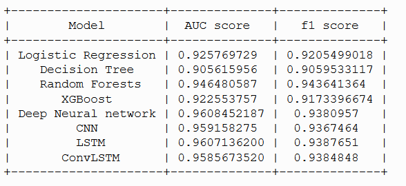
AUC score of logistic regression model is : 0.925

Logistic回归模型的AUC得分为0.925

F1 score of logistic regression model is : 0.920

Logistic回归模型的F1得分是： 0.920

from sklearn.model_selection import GridSearchCV
from sklearn.linear_model import SGDClassifier
#Hyperparameter tuning of sgd with log loss(i.e logistic regression).grid = {'alpha': [1e-4, 1e-3, 1e-2, 1e-1, 1e0, 1e1, 1e2, 1e3],'max_iter': [100,500,1000], 'loss': ['log'], # logistic regression,'penalty': ['l2'],}sgd=SGDClassifier()
sgd_cv=GridSearchCV(sgd,grid,cv=10,n_jobs=5,verbose=10)
sgd_cv.fit(X_train,y_train)
print("tuned hyperparameters :(best parameters) ",sgd_cv.best_params_)
print("accuracy :",sgd_cv.best_score_)sgd = SGDClassifier(alpha = 0.0001, loss ='log', max_iter = 100, penalty = 'l2')
sgd.fit(X_train,y_train)

决策树 ： (Decision Tree :)

AUC score of decision tree model is : 0.905

决策树模型的AUC得分是： 0.905

F1 score of decision tree model is : 0.905

决策树模型的F1得分是： 0.905

#Hyperparameter tuning of DecisionTree.
from sklearn.model_selection import GridSearchCV
from sklearn.tree import DecisionTreeClassifiergrid={'criterion':['gini','entropy'],'max_depth':[90,100,110],'min_samples_split':[8,10,12]}# l1 lasso l2 ridge
tree=DecisionTreeClassifier()
tree_cv=GridSearchCV(tree,grid,cv=10,n_jobs=5,verbose=10)
tree_cv.fit(X_train,y_train)print("tuned hyperparameters :(best parameters) ",tree_cv.best_params_)
print("accuracy :",tree_cv.best_score_)tree = DecisionTreeClassifier(criterion = 'entropy', max_depth = 90, min_samples_split = 12)
tree.fit(X_train,y_train)

随机森林： (Random Forest :)

AUC score of random forest model is : 0.946

随机森林模型的AUC分数是： 0.946

F1 score of random forest model is : 0.943

随机森林模型的F1得分是： 0.943

#Hyperparameter tuning of RandomForest.
from sklearn.model_selection import GridSearchCV
from sklearn.ensemble import RandomForestClassifiergrid={'n_estimators':[100,200],'max_depth': [10,20,50],'min_samples_split': [2, 5, 10],'min_samples_leaf': [2, 4]}
randomforest=RandomForestClassifier()
randomforest_cv=GridSearchCV(randomforest,grid,cv=8,n_jobs=5,verbose=10)
randomforest_cv.fit(X_train,y_train)print("tuned hyperparameters :(best parameters) ",randomforest_cv.best_params_)
print("accuracy :",randomforest_cv.best_score_)randomforest = RandomForestClassifier(max_depth= 50, min_samples_leaf= 2, min_samples_split= 2, n_estimators= 200)
randomforest.fit(X_train,y_train)

XGBoost： (XGBoost :)

AUC score of xgboost model is : 0.933

xgboost模型的AUC得分是： 0.933

F1 score of xgboost model is : 0.929

xgboost模型的F1得分是： 0.929

#Hyperparameter tuning of xgboost.
from sklearn.model_selection import GridSearchCV
import xgboost as xgbgrid={"learning_rate"    : [0.05, 0.10 ] ,"max_depth"        : [ 3, 4, 5],"min_child_weight" : [ 1, 3,],"gamma"            : [ 0.0, 0.1, 0.3 ],"colsample_bytree" : [ 0.3,0.5 , 0.7 ] }
xg=xgb.XGBClassifier()
xg_cv=GridSearchCV(xg,grid,cv=8,n_jobs=5,verbose=10)
xg_cv.fit(X_train,y_train)print("tuned hyperparameters :(best parameters) ",xg_cv.best_params_)
print("accuracy :",xg_cv.best_score_)xg = xgb.XGBClassifier(colsample_bytree= 0.5, gamma= 0.3, learning_rate= 0.1, max_depth= 5,min_child_weight= 1)
xg.fit(X_train,y_train)

深度神经网络： (Deep Neural network :)

AUC score of xgboost model is : 0.960

xgboost模型的AUC得分是： 0.960

F1 score of xgboost model is : 0.938

F1分数 xgboost型号为：0.938

tf.keras.backend.clear_session()
model = tf.keras.models.Sequential()
#Input layer
input_layer = tf.keras.Input(shape=(82,))#Dense hidden layer
layer1 = tf.keras.layers.Dense(512,activation='relu')(input_layer)
layer2 = tf.keras.layers.Dense(256,activation='relu')(layer1)
layer3 = tf.keras.layers.Dense(128,activation='relu')(layer2)
layer4 = tf.keras.layers.Dense(64,activation='relu')(layer3)
layer5 = tf.keras.layers.Dense(32,activation='relu')(layer4)#output layer
output = tf.keras.layers.Dense(2,activation='softmax',kernel_initializer=tf.initializers.he_uniform())(layer5)#Creating a model
model = tf.keras.Model(inputs=input_layer,outputs=output)#adam optimizer
optimizer = tf.keras.optimizers.Adam(learning_rate=0.001, beta_1=0.9, beta_2=0.999, epsilon=1e-07, amsgrad=False,name='Adam')es = EarlyStopping(monitor='val_loss', mode='min',verbose=1,patience=2,restore_best_weights=True)tensorboard_callback = tf.keras.callbacks.TensorBoard(log_dir='./graph002',histogram_freq=1, write_graph=True,write_grads=True)#changes learning rate if val_auc is same or less than max val_auc
scheduler = ReduceLROnPlateau(monitor='val_auc', factor=0.9, patience=0, verbose=1,mode = 'max')model.compile(optimizer=optimizer, loss='categorical_crossentropy',metrics =[auc,f1])callback_list = [tensorboard_callback,scheduler,es]model.fit(X_train,y_train,epochs=100, validation_data=(X_cv,y_cv), batch_size=100, callbacks=callback_list)

有线电视新闻网 (CNN)

AUC score of xgboost model is : 0.959

AUC得分 xgboost型号为：0.959

F1 score of xgboost model is : 0.936

xgboost模型的F1得分是： 0.936

tf.keras.backend.clear_session()input_layer = Input(shape=(X_train_1.shape[1],82),)
l_cov1= Conv1D(64, 5, activation='relu',padding='same')(input_layer)
l_cov2= Conv1D(32, 5, activation='relu',padding='same')(l_cov1)
dropout2 = Dropout(0.25)(l_cov2)
text_flat1 = Flatten(data_format='channels_last',name='other_data_flat')(dropout2)
dense1 = Dense(64,activation='relu')(text_flat1)#output layer
output = tf.keras.layers.Dense(2,activation='softmax')(dense1)#Creating a model
model = tf.keras.Model(inputs=input_layer,outputs=output)#adam optimizer
optimizer = tf.keras.optimizers.Adam(learning_rate=0.001, beta_1=0.9, beta_2=0.999, epsilon=1e-07, amsgrad=False,name='Adam')tensorboard_callback = tf.keras.callbacks.TensorBoard(log_dir='./graph003',histogram_freq=1, write_graph=True,write_grads=True)#changes learning rate if val_auc is same or less than max val_auc
scheduler = ReduceLROnPlateau(monitor='val_auc', factor=0.9, patience=0, verbose=1,mode = 'max')es = EarlyStopping(monitor='val_loss', mode='min',verbose=1,patience=2,restore_best_weights=True)model.compile(optimizer=optimizer, loss='categorical_crossentropy',metrics =[auc,f1])callback_list = [tensorboard_callback,scheduler,es]model.fit(X_train_1,y_train_1,epochs=100, validation_data=(X_cv_1,y_cv_1), batch_size=100, callbacks=callback_list)

LSTM： (LSTM :)

AUC score of xgboost model is : 0.960

xgboost模型的AUC得分是： 0.960

F1 score of xgboost model is : 0.938

F1分数 xgboost型号为：0.938

tf.keras.backend.clear_session()input_layer = Input(shape=(1,82),)
lstm1= LSTM(128, activation='relu')(input_layer)
text_flat = Flatten(data_format='channels_last',name='Flatten1')(lstm1)
dense1 = Dense(64,activation='relu')(text_flat)
dropout2 = Dropout(0.25)(text_flat)
#output layer
output = tf.keras.layers.Dense(2,activation='softmax')(dropout2)#Creating a model
model = tf.keras.Model(inputs=input_layer,outputs=output)#Callbacks
#history_own = LossHistory()#adam optimizer
optimizer = tf.keras.optimizers.Adam(learning_rate=0.001, beta_1=0.9, beta_2=0.999, epsilon=1e-07, amsgrad=False,name='Adam')tensorboard_callback = tf.keras.callbacks.TensorBoard(log_dir='./graph012',histogram_freq=1, write_graph=True,write_grads=True)es = EarlyStopping(monitor='val_loss', mode='min',verbose=1,patience=2,restore_best_weights=True)scheduler = ReduceLROnPlateau(monitor='val_auc', factor=0.9, patience=0, verbose=1,mode = 'max')model.compile(optimizer=optimizer, loss='categorical_crossentropy',metrics =[auc,f1])callback_list = [tensorboard_callback,scheduler,es]model.fit(X_train_1,y_train_1,epochs=30, validation_data=(X_cv_1,y_cv_1), batch_size=100, callbacks=callback_list)

转换STM (ConvLSTM :)

AUC score of xgboost model is : 0.958

xgboost模型的AUC得分是： 0.958

F1 score of xgboost model is : 0.938

F1分数 xgboost型号为：0.938

tf.keras.backend.clear_session()input_layer = Input(shape=(X_train_1.shape[1],82),)
l_cov1= Conv1D(64, 5, activation='relu',padding='same')(input_layer)
l_cov2= Conv1D(32, 5, activation='relu',padding='same')(l_cov1)
lstm1= LSTM(128, activation='relu')(l_cov2)
dropout =Dropout(0.25)(lstm1)
text_flat = Flatten(data_format='channels_last',name='Flatten1')(dropout)
dense1 = Dense(64,activation='relu')(text_flat)
#output layer
output = tf.keras.layers.Dense(2,activation='softmax')(dense1)#Creating a model
model = tf.keras.Model(inputs=input_layer,outputs=output)#adam optimizer
optimizer = tf.keras.optimizers.Adam(learning_rate=0.0001, beta_1=0.9, beta_2=0.999, epsilon=1e-07, amsgrad=False,name='Adam')tensorboard_callback = tf.keras.callbacks.TensorBoard(log_dir='./graph0011',histogram_freq=1, write_graph=True,write_grads=True)scheduler = ReduceLROnPlateau(monitor='val_auc', factor=0.9, patience=0, verbose=1,mode = 'max')es = EarlyStopping(monitor='val_loss', mode='min',verbose=1,patience=2,restore_best_weights=True)model.compile(optimizer=optimizer, loss='categorical_crossentropy',metrics =[auc,f1])callback_list = [tensorboard_callback,scheduler,es]model.fit(X_train_1,y_train_1,epochs=100, validation_data=(X_cv_1,y_cv_1), batch_size=80, callbacks=callback_list)

结果： (Results:)

• We can observe that LSTM dominates when auc score is considered.我们可以观察到，考虑到auc分数时，LSTM占主导地位。
• We can observe that random forest dominates when f1 score is considered.我们可以观察到，考虑f1分数时，随机森林占主导地位。

结论： (Conclusion:)

This was my first self-case study and my first medium article, I hope you enjoyed reading through it. I got to learn lot of techniques while working on this case study. I thank AppliedAI and my mentor who helped me throughout this case study.

这是我的第一份自我案例研究，也是我的第一篇中篇文章，希望您喜欢阅读。 在进行此案例研究时，我必须学习很多技术。 我感谢AppliedAI和我的导师在整个案例研究中为我提供了帮助。

This concludes my work. Thank you for reading!

我的工作到此结束。 感谢您的阅读！