神经网络，流形和拓扑Neural Networks, Manifolds, and Topology

Recently, there’s been a great deal of excitement and interest in deep neural networks because they’ve achieved breakthrough results in areas such as computer vision.1

However, there remain a number of concerns about them. One is that it can be quite challenging to understand what a neural network is really doing. If one trains it well, it achieves high quality results, but it is challenging to understand how it is doing so. If the network fails, it is hard to understand what went wrong.

While it is challenging to understand the behavior of deep neural networks in general, it turns out to be much easier to explore low-dimensional deep neural networks – networks that only have a few neurons in each layer. In fact, we can create visualizations to completely understand the behavior and training of such networks. This perspective will allow us to gain deeper intuition about the behavior of neural networks and observe a connection linking neural networks to an area of mathematics called topology.

A number of interesting things follow from this, including fundamental lower-bounds on the complexity of a neural network capable of classifying certain datasets.

A Simple Example

Let’s begin with a very simple dataset, two curves on a plane. The network will learn to classify points as belonging to one or the other.

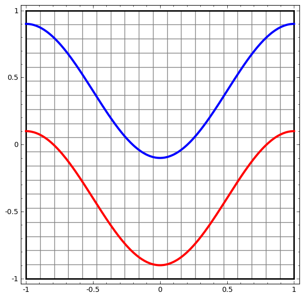
The obvious way to visualize the behavior of a neural network – or any classification algorithm, for that matter – is to simply look at how it classifies every possible data point.

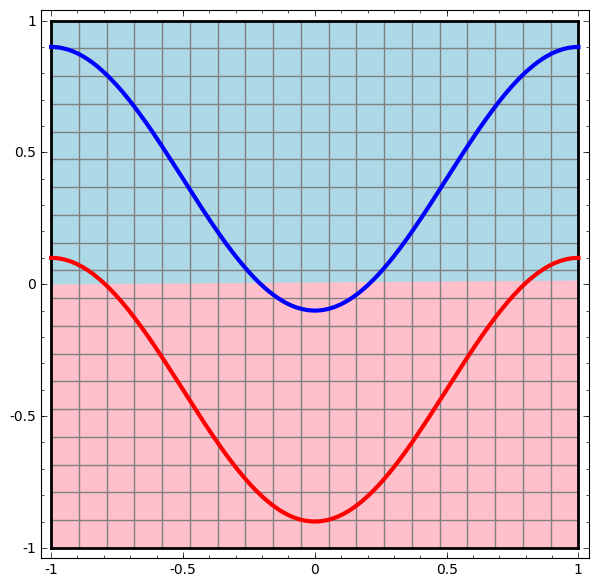
We’ll start with the simplest possible class of neural network, one with only an input layer and an output layer. Such a network simply tries to separate the two classes of data by dividing them with a line.

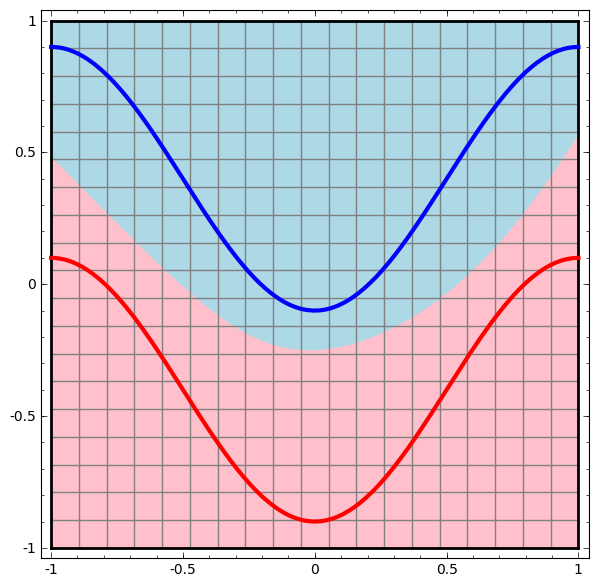
That sort of network isn’t very interesting. Modern neural networks generally have multiple layers between their input and output, called “hidden” layers. At the very least, they have one.

Diagram of a simple network from Wikipedia

As before, we can visualize the behavior of this network by looking at what it does to different points in its domain. It separates the data with a more complicated curve than a line.

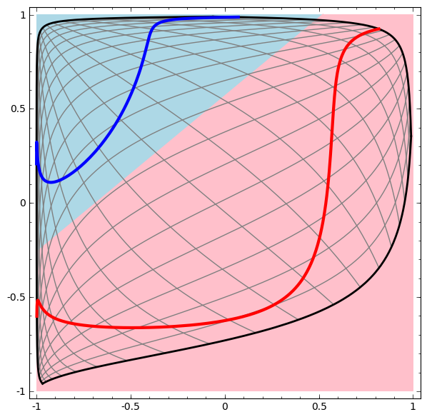
With each layer, the network transforms the data, creating a new representation.2 We can look at the data in each of these representations and how the network classifies them. When we get to the final representation, the network will just draw a line through the data (or, in higher dimensions, a hyperplane).

In the previous visualization, we looked at the data in its “raw” representation. You can think of that as us looking at the input layer. Now we will look at it after it is transformed by the first layer. You can think of this as us looking at the hidden layer.

Each dimension corresponds to the firing of a neuron in the layer.

The hidden layer learns a representation so that the data is linearly separable

Continuous Visualization of Layers

In the approach outlined in the previous section, we learn to understand networks by looking at the representation corresponding to each layer. This gives us a discrete list of representations.

The tricky part is in understanding how we go from one to another. Thankfully, neural network layers have nice properties that make this very easy.

There are a variety of different kinds of layers used in neural networks. We will talk about tanh layers for a concrete example. A tanh layer tanh(Wx+b) consists of:

A linear transformation by the “weight” matrix W
A translation by the vector b
Point-wise application of tanh.

We can visualize this as a continuous transformation, as follows:

Gradually applying a neural network layer

The story is much the same for other standard layers, consisting of an affine transformation followed by pointwise application of a monotone activation function.

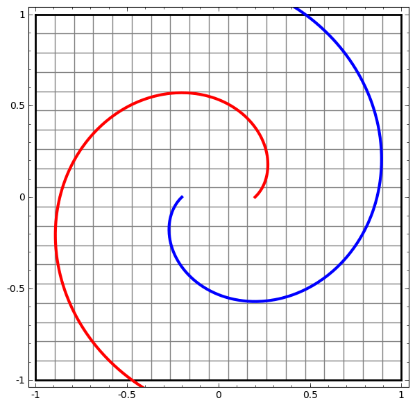
We can apply this technique to understand more complicated networks. For example, the following network classifies two spirals that are slightly entangled, using four hidden layers. Over time, we can see it shift from the “raw” representation to higher level ones it has learned in order to classify the data. While the spirals are originally entangled, by the end they are linearly separable.

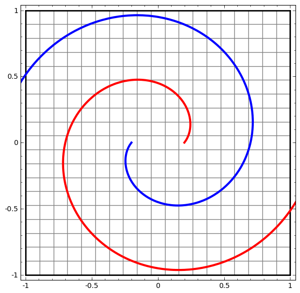
On the other hand, the following network, also using multiple layers, fails to classify two spirals that are more entangled.

It is worth explicitly noting here that these tasks are only somewhat challenging because we are using low-dimensional neural networks. If we were using wider networks, all this would be quite easy.

(Andrej Karpathy has made a nice demo based on ConvnetJS that allows you to interactively explore networks with this sort of visualization of training!)

Topology of tanh Layers

Each layer stretches and squishes space, but it never cuts, breaks, or folds it. Intuitively, we can see that it preserves topological properties. For example, a set will be connected afterwards if it was before (and vice versa).

Transformations like this, which don’t affect topology, are called homeomorphisms. Formally, they are bijections that are continuous functions both ways.

Theorem: Layers with N inputs and N outputs are homeomorphisms, if the weight matrix, W, is non-singular. (Though one needs to be careful about domain and range.)

Proof: Let’s consider this step by step:

Let’s assume W has a non-zero determinant. Then it is a bijective linear function with a linear inverse. Linear functions are continuous. So, multiplying by W is a homeomorphism.
Translations are homeomorphisms
tanh (and sigmoid and softplus but not ReLU) are continuous functions with continuous inverses. They are bijections if we are careful about the domain and range we consider. Applying them pointwise is a homemorphism

Thus, if W has a non-zero determinant, our layer is a homeomorphism. ∎

This result continues to hold if we compose arbitrarily many of these layers together.

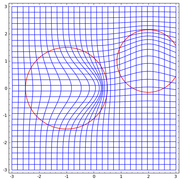
Topology and Classification

AA is red, BB is blue

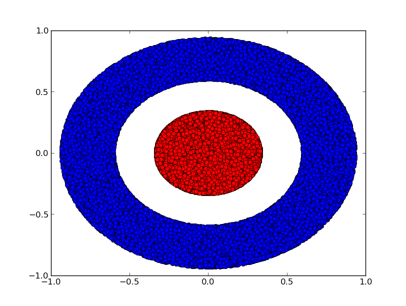
Consider a two dimensional dataset with two classes A,B⊂R2:

A = {x | d (x, 0) < 1 / 3}

B = {x | 2 / 3 < d (x, 0) < 1}

Claim: It is impossible for a neural network to classify this dataset without having a layer that has 3 or more hidden units, regardless of depth.

As mentioned previously, classification with a sigmoid unit or a softmax layer is equivalent to trying to find a hyperplane (or in this case a line) that separates A and B in the final represenation. With only two hidden units, a network is topologically incapable of separating the data in this way, and doomed to failure on this dataset.

In the following visualization, we observe a hidden representation while a network trains, along with the classification line. As we watch, it struggles and flounders trying to learn a way to do this.

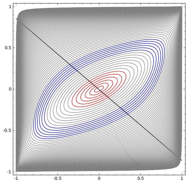
For this network, hard work isn’t enough.

In the end it gets pulled into a rather unproductive local minimum. Although, it’s actually able to achieve ∼80% classification accuracy.

This example only had one hidden layer, but it would fail regardless.

Proof: Either each layer is a homeomorphism, or the layer’s weight matrix has determinant 0. If it is a homemorphism, A is still surrounded by B, and a line can’t separate them. But suppose it has a determinant of 0: then the dataset gets collapsed on some axis. Since we’re dealing with something homeomorphic to the original dataset, A is surrounded by B, and collapsing on any axis means we will have some points of A and B mix and become impossible to distinguish between. ∎

If we add a third hidden unit, the problem becomes trivial. The neural network learns the following representation:

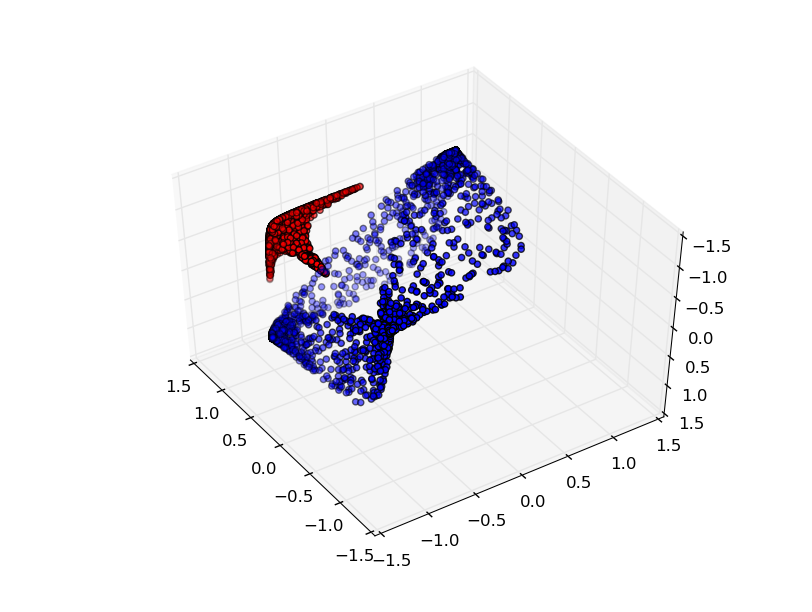
With this representation, we can separate the datasets with a hyperplane.

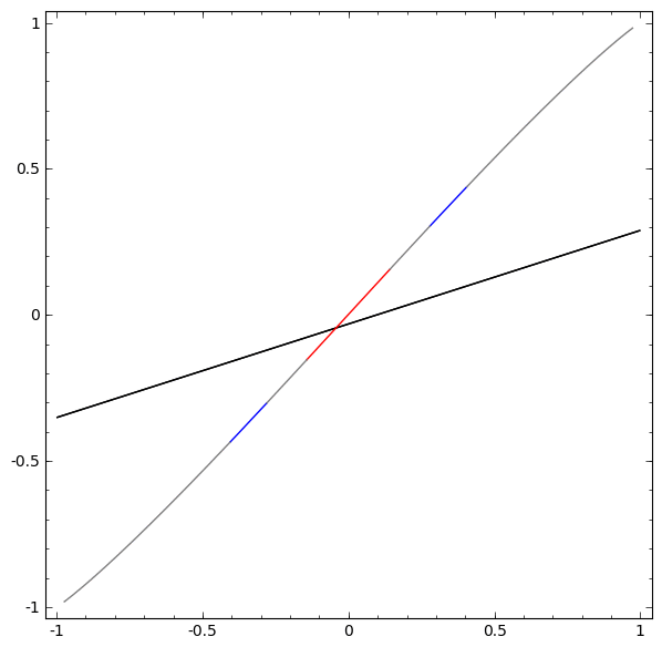
To get a better sense of what’s going on, let’s consider an even simpler dataset that’s 1-dimensional:

A = [- 1 3, 1 3]

B = [- 1, - 2 3] \cup [2 3, 1]

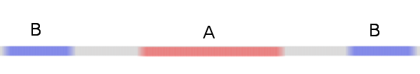
Without using a layer of two or more hidden units, we can’t classify this dataset. But if we use one with two units, we learn to represent the data as a nice curve that allows us to separate the classes with a line:

What’s happening? One hidden unit learns to fire when x>−12 and one learns to fire when x>12. When the first one fires, but not the second, we know that we are in A.

The Manifold Hypothesis

Is this relevant to real world data sets, like image data? If you take the manifold hypothesis really seriously, I think it bears consideration.

The manifold hypothesis is that natural data forms lower-dimensional manifolds in its embedding space. There are both theoretical3 and experimental4 reasons to believe this to be true. If you believe this, then the task of a classification algorithm is fundamentally to separate a bunch of tangled manifolds.

In the previous examples, one class completely surrounded another. However, it doesn’t seem very likely that the dog image manifold is completely surrounded by the cat image manifold. But there are other, more plausible topological situations that could still pose an issue, as we will see in the next section.

Links And Homotopy

Another interesting dataset to consider is two linked tori, A and B.

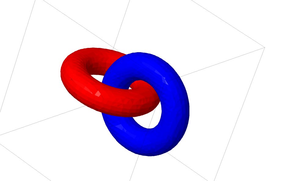
Much like the previous datasets we considered, this dataset can’t be separated without using n+1 dimensions, namely a 4th dimension.

Links are studied in knot theory, an area of topology. Sometimes when we see a link, it isn’t immediately obvious whether it’s an unlink (a bunch of things that are tangled together, but can be separated by continuous deformation) or not.

A relatively simple unlink.

If a neural network using layers with only 3 units can classify it, then it is an unlink. (Question: Can all unlinks be classified by a network with only 3 units, theoretically?)

From this knot perspective, our continuous visualization of the representations produced by a neural network isn’t just a nice animation, it’s a procedure for untangling links. In topology, we would call it an ambient isotopy between the original link and the separated ones.

Formally, an ambient isotopy between manifolds A and B is a continuous function F:[0,1]×X→Y such that each Ft is a homeomorphism from X to its range, F0 is the identity function, and F1 maps A to B. That is, Ft continuously transitions from mapping A to itself to mapping A to B.

Theorem: There is an ambient isotopy between the input and a network layer’s representation if: a) W isn’t singular, b) we are willing to permute the neurons in the hidden layer, and c) there is more than 1 hidden unit.

Proof: Again, we consider each stage of the network individually:

The hardest part is the linear transformation. In order for this to be possible, we need W to have a positive determinant. Our premise is that it isn’t zero, and we can flip the sign if it is negative by switching two of the hidden neurons, and so we can guarantee the determinant is positive. The space of positive determinant matrices is path-connected, so there exists p:[0,1]→GLn(R)5 such that p(0)=Id and p(1)=W. We can continually transition from the identity function to the W transformation with the function x→p(t)x, multiplying xat each point in time t by the continuously transitioning matrix p(t).

We can continually transition from the identity function to the b translation with the function x→x+tb.
We can continually transition from the identity function to the pointwise use of σ with the function: x→(1−t)x+tσ(x). ∎

I imagine there is probably interest in programs automatically discovering such ambient isotopies and automatically proving the equivalence of certain links, or that certain links are separable. It would be interesting to know if neural networks can beat whatever the state of the art is there.

(Apparently determining if knots are trivial is NP. This doesn’t bode well for neural networks.)

The sort of links we’ve talked about so far don’t seem likely to turn up in real world data, but there are higher dimensional generalizations. It seems plausible such things could exist in real world data.

Links and knots are 1-dimensional manifolds, but we need 4 dimensions to be able to untangle all of them. Similarly, one can need yet higher dimensional space to be able to unknot n-dimensional manifolds. All n-dimensional manifolds can be untangled in 2n+2 dimensions.6

(I know very little about knot theory and really need to learn more about what’s known regarding dimensionality and links. If we know a manifold can be embedded in n-dimensional space, instead of the dimensionality of the manifold, what limit do we have?)

The Easy Way Out

The natural thing for a neural net to do, the very easy route, is to try and pull the manifolds apart naively and stretch the parts that are tangled as thin as possible. While this won’t be anywhere close to a genuine solution, it can achieve relatively high classification accuracy and be a tempting local minimum.

It would present itself as very high derivatives on the regions it is trying to stretch, and sharp near-discontinuities. We know these things happen.7 Contractive penalties, penalizing the derivatives of the layers at data points, are the natural way to fight this.8

Since these sort of local minima are absolutely useless from the perspective of trying to solve topological problems, topological problems may provide a nice motivation to explore fighting these issues.

On the other hand, if we only care about achieving good classification results, it seems like we might not care. If a tiny bit of the data manifold is snagged on another manifold, is that a problem for us? It seems like we should be able to get arbitrarily good classification results despite this issue.

(My intuition is that trying to cheat the problem like this is a bad idea: it’s hard to imagine that it won’t be a dead end. In particular, in an optimization problem where local minima are a big problem, picking an architecture that can’t genuinely solve the problem seems like a recipe for bad performance.)

Better Layers for Manipulating Manifolds?

The more I think about standard neural network layers – that is, with an affine transformation followed by a point-wise activation function – the more disenchanted I feel. It’s hard to imagine that these are really very good for manipulating manifolds.

Perhaps it might make sense to have a very different kind of layer that we can use in composition with more traditional ones?

The thing that feels natural to me is to learn a vector field with the direction we want to shift the manifold:

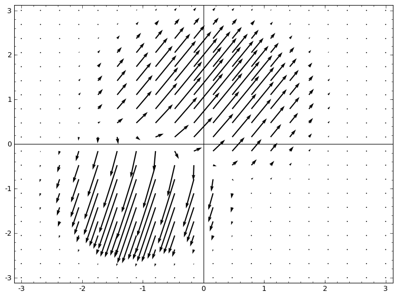
And then deform space based on it:

One could learn the vector field at fixed points (just take some fixed points from the training set to use as anchors) and interpolate in some manner. The vector field above is of the form:

F (x) = v 0 f 0 ( x ) + v 1 f 1 ( x ) 1 + f 0 ( x ) + f 1 ( x )

Where v0 and v1 are vectors and f0(x) and f1(x) are n-dimensional gaussians. This is inspired a bit by radial basis functions.

K-Nearest Neighbor Layers

I’ve also begun to think that linear separability may be a huge, and possibly unreasonable, amount to demand of a neural network. In some ways, it feels like the natural thing to do would be to use k-nearest neighbors (k-NN). However, k-NN’s success is greatly dependent on the representation it classifies data from, so one needs a good representation before k-NN can work well.

As a first experiment, I trained some MNIST networks (two-layer convolutional nets, no dropout) that achieved ∼1% test error. I then dropped the final softmax layer and used the k-NN algorithm. I was able to consistently achieve a reduction in test error of 0.1-0.2%.

Still, this doesn’t quite feel like the right thing. The network is still trying to do linear classification, but since we use k-NN at test time, it’s able to recover a bit from mistakes it made.

k-NN is differentiable with respect to the representation it’s acting on, because of the 1/distance weighting. As such, we can train a network directly for k-NN classification. This can be thought of as a kind of “nearest neighbor” layer that acts as an alternative to softmax.

We don’t want to feedforward our entire training set for each mini-batch because that would be very computationally expensive. I think a nice approach is to classify each element of the mini-batch based on the classes of other elements of the mini-batch, giving each one a weight of 1/(distance from classification target).9

Sadly, even with sophisticated architecture, using k-NN only gets down to 5-4% test error – and using simpler architectures gets worse results. However, I’ve put very little effort into playing with hyper-parameters.

Still, I really aesthetically like this approach, because it seems like what we’re “asking” the network to do is much more reasonable. We want points of the same manifold to be closer than points of others, as opposed to the manifolds being separable by a hyperplane. This should correspond to inflating the space between manifolds for different categories and contracting the individual manifolds. It feels like simplification.

Conclusion

Topological properties of data, such as links, may make it impossible to linearly separate classes using low-dimensional networks, regardless of depth. Even in cases where it is technically possible, such as spirals, it can be very challenging to do so.

To accurately classify data with neural networks, wide layers are sometimes necessary. Further, traditional neural network layers do not seem to be very good at representing important manipulations of manifolds; even if we were to cleverly set weights by hand, it would be challenging to compactly represent the transformations we want. New layers, specifically motivated by the manifold perspective of machine learning, may be useful supplements.

(This is a developing research project. It’s posted as an experiment in doing research openly. I would be delighted to have your feedback on these ideas: you can comment inline or at the end. For typos, technical errors, or clarifications you would like to see added, you are encouraged to make a pull request on github.)

Acknowledgments

Thank you to Yoshua Bengio, Michael Nielsen, Dario Amodei, Eliana Lorch, Jacob Steinhardt, and Tamsyn Waterhouse for their comments and encouragement.

This seems to have really kicked off with Krizhevsky et al., (2012), who put together a lot of different pieces to achieve outstanding results. Since then there’s been a lot of other exciting work.↩
These representations, hopefully, make the data “nicer” for the network to classify. There has been a lot of work exploring representations recently. Perhaps the most fascinating has been in Natural Language Processing: the representations we learn of words, called word embeddings, have interesting properties. See Mikolov et al. (2013), Turian et al. (2010), and,Richard Socher’s work. To give you a quick flavor, there is a very nice visualizationassociated with the Turian paper.↩
A lot of the natural transformations you might want to perform on an image, like translating or scaling an object in it, or changing the lighting, would form continuous curves in image space if you performed them continuously.↩
Carlsson et al. found that local patches of images form a klein bottle.↩
GLn(R) is the set of invertible n×n matrices on the reals, formally called the general linear group of degree n.↩
This result is mentioned in Wikipedia’s subsection on Isotopy versions.↩
See Szegedy et al., where they are able to modify data samples and find slight modifications that cause some of the best image classification neural networks to misclasify the data. It’s quite troubling.↩
Contractive penalties were introduced in contractive autoencoders. See Rifai et al. (2011).↩
I used a slightly less elegant, but roughly equivalent algorithm because it was more practical to implement in Theano: feedforward two different batches at the same time, and classify them based on each other.↩

from: http://colah.github.io/posts/2014-03-NN-Manifolds-Topology/