文章目录

1. 通过网格搜索完善模型
- 1.1 数据导入
- 1.2 拆分数据为训练集和测试集
- 1.3 拟合决策树模型
- 1.4 使用网络搜索完善模型
- 1.5 交叉验证可视化
- 1.5 总结

机器学习 | 目录

监督学习 | ID3 决策树原理及Python实现

监督学习 | ID3 & C4.5 决策树原理

监督学习 | CART 分类回归树原理

监督学习 | 决策树之Sklearn实现

监督学习 | 决策树之网络搜索

1. 通过网格搜索完善模型

在本文中，我们将为决策树模型拟合一些样本数据。这个初始模型会过拟合。然后，我们将使用网格搜索为这个模型找到更好的参数，以减少过拟合。

首先，导入所需要的库：

%matplotlib inline
import pandas as pd
import numpy as np
import matplotlib.pyplot as plt

1.1 数据导入

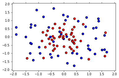
首先定义一个函数用于读取 csv 数据并进行可视化：

def load_pts(csv_name):data = np.asarray(pd.read_csv(csv_name, header=None))X = data[:,0:2]y = data[:,2]plt.scatter(X[np.argwhere(y==0).flatten(),0], X[np.argwhere(y==0).flatten(),1],s = 50, color = 'blue', edgecolor = 'k')plt.scatter(X[np.argwhere(y==1).flatten(),0], X[np.argwhere(y==1).flatten(),1],s = 50, color = 'red', edgecolor = 'k')plt.xlim(-2.05,2.05)plt.ylim(-2.05,2.05)plt.grid(False)plt.tick_params(axis='x',which='both',bottom='off',top='off')return X,yX, y = load_pts('Data/data.csv')
plt.show()

1.2 拆分数据为训练集和测试集

from sklearn.model_selection import train_test_split
from sklearn.metrics import f1_score, make_scorer#Fixing a random seed
import random
random.seed(42)# Split the data into training and testing sets
X_train, X_test, y_train, y_test = train_test_split(X, y, test_size=0.2, random_state=42)

1.3 拟合决策树模型

from sklearn.tree import DecisionTreeClassifier# Define the model (with default hyperparameters)
clf = DecisionTreeClassifier(random_state=42)# Fit the model
clf.fit(X_train, y_train)# Make predictions
train_predictions = clf.predict(X_train)
test_predictions = clf.predict(X_test)

现在我们来可视化模型，并测试 f1_score，首先定义可视化函数：

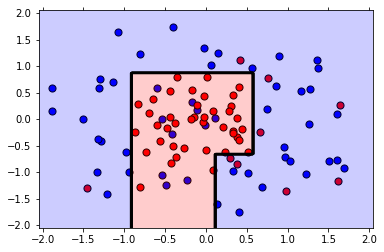
def plot_model(X, y, clf):# 绘制两类点的散点图plt.scatter(X[np.argwhere(y==0).flatten(),0],X[np.argwhere(y==0).flatten(),1],s = 50, color = 'blue', edgecolor = 'k')plt.scatter(X[np.argwhere(y==1).flatten(),0],X[np.argwhere(y==1).flatten(),1],s = 50, color = 'red', edgecolor = 'k')# 图形设置plt.xlim(-2.05,2.05)plt.ylim(-2.05,2.05)plt.grid(False)plt.tick_params(axis='x',which='both',bottom='off',top='off')# 利用 np.meshgrid(r,r) 生成一个平面对于的横纵坐标r = np.linspace(-2.1,2.1,300)s,t = np.meshgrid(r,r)# 将坐标转换为与决策树的训练集相同格式s = np.reshape(s,(np.size(s),1))t = np.reshape(t,(np.size(t),1))h = np.concatenate((s,t),1)# 对平面上的每一个点进行预测类别z = clf.predict(h)# 将横纵坐标及对应类别转换为矩阵形式s = s.reshape((np.size(r),np.size(r)))t = t.reshape((np.size(r),np.size(r)))z = z.reshape((np.size(r),np.size(r)))# 利用 plt.contourf 绘制不同等高面plt.contourf(s,t,z,colors = ['blue','red'],alpha = 0.2,levels = range(-1,2))# 绘制等高面边缘if len(np.unique(z)) > 1:plt.contour(s,t,z,colors = 'k', linewidths = 2)plt.show()

plot_model(X, y, clf)
print('The Training F1 Score is', f1_score(train_predictions, y_train))
print('The Testing F1 Score is', f1_score(test_predictions, y_test))

The Training F1 Score is 1.0
The Testing F1 Score is 0.7000000000000001

训练集得分为 1 ，而测试集得分为 0.7，可以看出当前模型有些过拟合，下面我们通过网络搜索来优化参数。

1.4 使用网络搜索完善模型

现在，我们将执行以下步骤：

1.首先，定义一些参数来执行网格搜索：max_depth, min_samples_leaf, 和 min_samples_split。

2.使用f1_score，为模型制作记分器。

3.使用参数和记分器，在分类器上执行网格搜索。

4.将数据拟合到新的分类器中。

5.绘制模型并找到 f1_score。

6.如果模型不太好，则更改参数的范围并再次拟合。

from sklearn.metrics import make_scorer
from sklearn.model_selection import GridSearchCVclf = DecisionTreeClassifier(random_state=42)# 生成参数列表
parameters = {'max_depth':[2,4,6,8,10],'min_samples_leaf':[2,4,6,8,10], 'min_samples_split':[2,4,6,8,10]}# 定义计分器
scorer = make_scorer(f1_score)# 生成网络搜索器
grid_obj = GridSearchCV(clf, parameters, scoring=scorer)# 拟合网络搜索器
grid_fit = grid_obj.fit(X_train, y_train)# 获得最佳决策树模型
best_clf = grid_fit.best_estimator_# 对最佳模型进行拟合
best_clf.fit(X_train, y_train)# 对测试集和训练集进行预测
best_train_predictions = best_clf.predict(X_train)
best_test_predictions = best_clf.predict(X_test)# 计算测试集得分和训练集得分
print('The training F1 Score is', f1_score(best_train_predictions, y_train))
print('The testing F1 Score is', f1_score(best_test_predictions, y_test))# 模型可视化
plot_model(X, y, best_clf)# 查看最佳模型的参数设置
best_clf

The training F1 Score is 0.8148148148148148
The testing F1 Score is 0.8

DecisionTreeClassifier(class_weight=None, criterion='gini', max_depth=4,max_features=None, max_leaf_nodes=None,min_impurity_decrease=0.0, min_impurity_split=None,min_samples_leaf=2, min_samples_split=2,min_weight_fraction_leaf=0.0, presort=False,random_state=42, splitter='best')

由此可以看出，最佳参数为：

max_depth=4

min_samples_leaf=2

min_samples_split=2

且相对于第一个图，边界更为简单，这意味着它不太可能过拟合。

1.5 交叉验证可视化

首先看一下不同参数下的信息：

results = pd.DataFrame(grid_obj.cv_results_)
results.T

	0	1	2	3	4	5	6	7	8	9	...	115	116	117	118	119	120	121	122	123	124
mean_fit_time	0.000536919	0.000609636	0.00067091	0.0005006	0.000532627	0.000538429	0.00162276	0.000725031	0.000346661	0.000960668	...	0.000691652	0.000363668	0.00054733	0.000414769	0.000365416	0.000314713	0.000483354	0.000389099	0.000378688	0.000585318
std_fit_time	7.36079e-05	0.000217965	0.000120917	7.64067e-05	0.000118579	0.000201879	0.00125017	0.000257437	2.95338e-05	0.000841452	...	0.00027542	3.20732e-05	0.000166427	5.31612e-05	2.22742e-05	5.03509e-06	0.000156771	0.000113168	6.09452e-05	0.000168713
mean_score_time	0.00124542	0.00209157	0.0011754	0.00118478	0.00127451	0.00132982	0.00173569	0.00158167	0.000804345	0.00165256	...	0.00107495	0.000776132	0.0010496	0.00107972	0.000799974	0.000889381	0.00097998	0.000957966	0.00082167	0.00108504
std_score_time	0.000460223	0.00131765	0.000217313	0.000175357	0.000274129	0.000684221	0.00012585	0.000531796	2.83336e-05	0.00103978	...	0.000327278	1.61637e-05	0.000181963	0.000226213	3.18651e-05	0.00015253	0.000282182	0.00014771	5.40954e-05	0.00015636
param_max_depth	2	2	2	2	2	2	2	2	2	2	...	10	10	10	10	10	10	10	10	10	10
param_min_samples_leaf	2	2	2	2	2	4	4	4	4	4	...	8	8	8	8	8	10	10	10	10	10
param_min_samples_split	2	4	6	8	10	2	4	6	8	10	...	2	4	6	8	10	2	4	6	8	10
params	{'max_depth': 2, 'min_samples_leaf': 2, 'min_s...	{'max_depth': 2, 'min_samples_leaf': 2, 'min_s...	{'max_depth': 2, 'min_samples_leaf': 2, 'min_s...	{'max_depth': 2, 'min_samples_leaf': 2, 'min_s...	{'max_depth': 2, 'min_samples_leaf': 2, 'min_s...	{'max_depth': 2, 'min_samples_leaf': 4, 'min_s...	{'max_depth': 2, 'min_samples_leaf': 4, 'min_s...	{'max_depth': 2, 'min_samples_leaf': 4, 'min_s...	{'max_depth': 2, 'min_samples_leaf': 4, 'min_s...	{'max_depth': 2, 'min_samples_leaf': 4, 'min_s...	...	{'max_depth': 10, 'min_samples_leaf': 8, 'min_...	{'max_depth': 10, 'min_samples_leaf': 8, 'min_...	{'max_depth': 10, 'min_samples_leaf': 8, 'min_...	{'max_depth': 10, 'min_samples_leaf': 8, 'min_...	{'max_depth': 10, 'min_samples_leaf': 8, 'min_...	{'max_depth': 10, 'min_samples_leaf': 10, 'min...	{'max_depth': 10, 'min_samples_leaf': 10, 'min...	{'max_depth': 10, 'min_samples_leaf': 10, 'min...	{'max_depth': 10, 'min_samples_leaf': 10, 'min...	{'max_depth': 10, 'min_samples_leaf': 10, 'min...
split0_test_score	0.642857	0.642857	0.642857	0.642857	0.642857	0.642857	0.642857	0.642857	0.642857	0.642857	...	0.642857	0.642857	0.642857	0.642857	0.642857	0.642857	0.642857	0.642857	0.642857	0.642857
split1_test_score	0.764706	0.764706	0.764706	0.764706	0.764706	0.764706	0.764706	0.764706	0.764706	0.764706	...	0.5	0.5	0.5	0.5	0.5	0.5	0.5	0.5	0.5	0.5
split2_test_score	0.709677	0.709677	0.709677	0.709677	0.709677	0.709677	0.709677	0.709677	0.709677	0.709677	...	0.714286	0.714286	0.714286	0.714286	0.714286	0.666667	0.666667	0.666667	0.666667	0.666667
mean_test_score	0.705698	0.705698	0.705698	0.705698	0.705698	0.705698	0.705698	0.705698	0.705698	0.705698	...	0.617857	0.617857	0.617857	0.617857	0.617857	0.602381	0.602381	0.602381	0.602381	0.602381
std_test_score	0.0501306	0.0501306	0.0501306	0.0501306	0.0501306	0.0501306	0.0501306	0.0501306	0.0501306	0.0501306	...	0.0889995	0.0889995	0.0889995	0.0889995	0.0889995	0.0737135	0.0737135	0.0737135	0.0737135	0.0737135
rank_test_score	14	14	14	14	14	14	14	14	14	14	...	42	42	42	42	42	62	62	62	62	62

14 rows × 125 columns

接着我们来看一下在不同的最大深度（max_depth）下，每片叶子的最小样本数（min_samples_leaf）和每次分裂的最小样本数（min_samples_split）对决策树模型的泛化性能的影响。

首先定义一个函数来绘制不同最大深度下的热力图（需安装 mglearn）：

def hotmap(max_depth, results):fliter = results[results['param_max_depth']==max_depth]scores = np.array(fliter['mean_test_score']).reshape(5, 5)mglearn.tools.heatmap(scores, xlabel='min_samples_split', xticklabels=parameters['min_samples_split'],ylabel='min_samples_leaf', yticklabels=parameters['min_samples_leaf'], cmap="viridis")

绘制到子图中：

import matplotlib.pyplot as plt
plt.figure(figsize=(20, 20))
plt
for i in [1,2,3,4,5]:plt.subplot(1,5,i, title='max_depth={}'.format(2*i))hotmap(2*i, results)

从图中可以看出，每次分裂的最小样本数（min_samples_split）对模型几乎没有影响，而随着最大深度（max_depth）的增加，模型得分逐渐降低。

1.5 总结

通过使用网格搜索，我们将 F1 分数从 0.7 提高到 0.8（同时我们失去了一些训练分数，但这没问题）。另外，如果你看绘制的图，第二个模型的边界更为简单，这意味着它不太可能过拟合。

监督学习 | 决策树之网络搜索相关推荐

机器学习 | 网络搜索及可视化
文章目录 1. 网络搜索 1.1 简单网络搜索 1.2 参数过拟合的风险与验证集 1.3 带交叉验证的网络搜索 1.3.1 Python 实现 1.3.2 Sklearn 实现 1.4 网络搜索可视化 ...
监督学习 | 决策树之Sklearn实现
文章目录 1. Sklearn中决策树的超参数 1.1 最大深度 max_depth 1.2 每片叶子的最小样本数 min_samples_leaf 1.3 每次分裂的最小样本数 min_sample ...
（转）【重磅】无监督学习生成式对抗网络突破，OpenAI 5大项目落地
[重磅]无监督学习生成式对抗网络突破,OpenAI 5大项目落地 [新智元导读]"生成对抗网络是切片面包发明以来最令人激动的事情!"LeCun前不久在Quroa答问时毫不加掩饰对生 ...
小技巧: 从开始菜单进行网络搜索
开始菜单的功能常常被忽视...... 只在寻找某个应用程序或进入控制面板的时候才想起它?事实上,它的本领可远不止这些. 今天小易就和大家分享的小技巧:从开始菜单进行网络搜索. 对 Windows 7 ...
决策树结合网格搜索交叉验证的例子
决策树结合网格搜索交叉验证如下是常见的模型评估的指标定义及决策树结合网格搜索交叉验证的例子.详见下文: 混淆矩阵: 准确率: 精准率(预测为正样本真实也是正例的比值,又称为查准率): 召回率(真实为 ...
phpsotrm怎么搜索功能_Windows 10 网络搜索设计太反人类？教你如何彻底关闭它
来源:太平洋电脑网我们知道微软在Windows 10中,特别加强了系统的搜索功能,但Windows 10的搜索的确很难称得上好用.抛开效率低下.呈现结果少.造成系统卡顿等老生常谈的问题不论,在功能设 ...
【网络搜索】学习资料
文章目录 1.综述 2.相关技术 3.课程 4. 论文 1.综述微软综述视频,较老但不过时 2.相关技术相关技术目录 3.课程北邮<网络搜索原理>2020 4. 论文 sigir
windows10搜索网络计算机,教你如何关闭Win10搜索的网络搜索功能
我们知道微软在 Win10 中,特别加强了系统的搜索功能,但 Win10 的搜索的确很难称得上好用.抛开效率低下.呈现结果少.造成系统卡顿等老生常谈的问题不论,在功能设计方面,Win10 搜索也有硬伤 ...
【华为云技术分享】自动网络搜索（NAS）在语义分割上的应用（二）
[摘要] 本文将介绍如何基于ProxylessNAS搜索semantic segmentation模型.最终搜索得到的模型结构可在CPU上达到36 fps. 随着自动网络搜索(Neural Archi ...