How to Visualize Your Recurrent Neural Network with Attention in Keras
Neural networks are taking over every part of our lives. In particular — thanks to deep learning — Siri can fetch you a taxi using your voice; and Google can enhance and organize your photos automagically. Here at Datalogue, we use deep learning to structurally and semantically understand data, allowing us to prepare it for use automatically.
Neural networks are massively successful in the domain of computer vision. Specifically, convolutional neural networks(CNNs) take images and extract relevant features from them by using small windows that travel over the image. This understanding can be leveraged to identify objects from your camera (Google Lens) and, in the future, even drive your car (NVIDIA).
The analogous neural network for text data is the recurrent neural network(RNN). This kind of network is designed for sequential data and applies the same function to the words or characters of the text. These models are successful in translation (Google Translate), speech recognition (Cortana) and language generation.
Dr. Yoshua Bengio from Université de Montréal believes that language is going to be the next challenge for neural networks. At Datalogue, we deal with tons of text data, and we are interested in helping the community solve this challenge.
In this tutorial, we will write an RNN in Keras that can translate human dates (“November 5, 2016”, “5th November 2016”) into a standard format (“2016–11–05”). In particular, we want to gain some intuition into how the neural network did this. We will leverage the concept of attention to generate a map (like that shown in Figure 1) that shows which input characters were important in predicting the output characters.
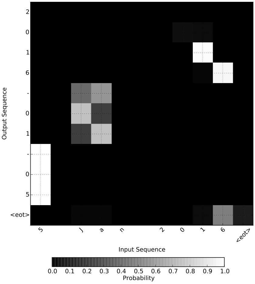
Figure 1: Attention map for the freeform date “5 Jan 2016”.We can see that the neural network used “16” to decide that the year was 2016, “Ja” to decide that the month was 01 and the first bit of the date to decide the day of the month.
What is in this Tutorial
We start off with some technical background material to get everyone on the same page and then move on to programming this thing! Throughout the tutorial, I will provide links to more advanced content.
If you want to directly jump to the code:
keras-attention - Visualizing RNNs using the attention mechanismgithub.com
What you need to know
To be able to jump into the coding part of this tutorial, it would be best if you have some familiarity with Python and Keras. You should have some familiarity of linear algebra, in particular that neural networks are just a few weight matrices with some non-linearities applied to it.
The intuition of RNNs and seq2seq models will be explained below.
Recurrent Neural Networks (RNN)
An RNN is a function that applies the same transformation (known as the RNN cell or step) to every element of a sequence. The output of an RNN layer is the output of the RNN cell applied on each element of the sequence. In the case of text, these are usually successive words or characters. In addition to this, RNN cells hold an internal memory that summarize the history of the sequence it has seen so far.
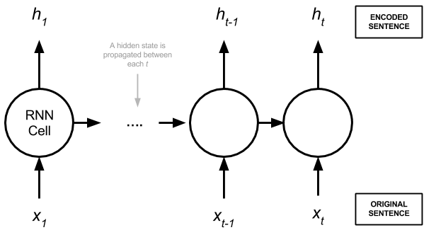
Figure 2: An example of an RNN Layer.The RNN Cell is applied to each element xi in the original sequence to get the corresponding element hi in the output sequence. The RNN cell uses a previous hidden state (propagated between the RNN cells) and the sequence element xi to do its calculations.
The output of the RNN layer is an encoded sequence, h, that can be manipulated and passed into another network. RNNs are incredibly flexible in their inputs and outputs:
- Many-to-One: use the complete input sequence to make a single prediction
h. - One-to-Many: transforming a single input to generate a sequence
h. - Many-to-Many: transforming the entire input sequence into another sequence.
In theory, the sequences in our training data need not be of the same length. In practice, we pad or truncate them to be of the same length to take advantage of the static computational graph in Tensorflow.
We will focus on #3 “Many-to-Many” also known as sequence-to-sequence (seq2seq).
Long sequences can be difficult to learn from in RNNs due to instabilities in gradient calculations during training. To solve this, the RNN cell is replaced by a gated cell like the gated recurrent unit (GRU) or the long-short term memory cell (LSTM). To learn more about LSTMs and gated units, I highly recommend reading Christopher Olah’s blog (it’s where I first started understanding the RNN cell). From now on, whenever we talk about RNNs, we are talking about a gated cell. Since Olah’s blog gives an intuitive introduction to LSTMs, we will use that.
A General Framework for seq2seq: The Encoder-Decoder Setup
Almost all neural network approaches to solving the seq2seq problem involve:
- Encoding the input sentences into some abstract representation.
- Manipulating this encoding.
- Decoding it to our target sequence.
Our encoders and decoders can be any kind and combination of neural networks. In practice, most people use RNNs for both the encoders and decoders.
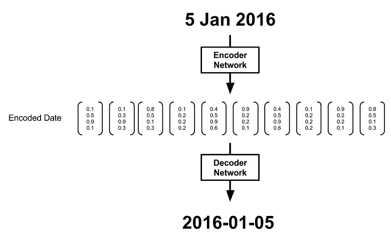
Figure 3: Set up of the encoder-decoder architecture.The encoder network processes the input sequence into an encoded sequence which is subsequently used by the decoder network to produce the output.
Figure 3 shows a simple encoder-decoder setup. The encoding step usually produces a sequence of vectors, h,corresponding to the sequence of characters in the input date, x. In an RNN encoder, each vector is generated by integrating information from the past sequence of vectors.
Before h is passed onto the decoder, we may choose to manipulate it in preparation for the decoder. For example, we might choose to only use the last encoding, as shown in Figure 4, since in theory, it is a summary of the whole sequence.
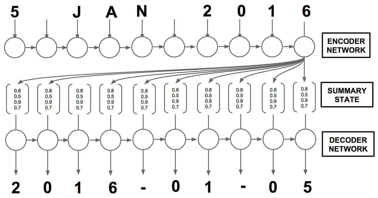
Figure 4: Use of a summary state in the encoder-decoder architecture.
Intuitively, this is similar to summarizing the whole input date into a single representation and then trying to decode that. While there may be enough information in this summary state for a classification problem like detecting sentiment (Many-to-One), it might be insufficient for an effective translation where it helps to consider the full sequence of hidden states (Figure 5).
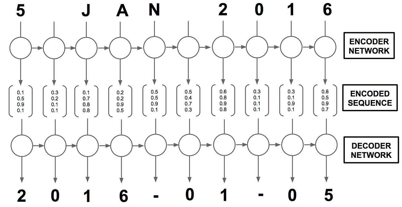
Figure 5: Use of the complete encoded sequence in the decoder network.
However, this is not how humans translate dates: We do not read the whole text and then independently write down the translation at each character. Intuitively, a person would understand that the characters “Jan” correspond to 1st month, “5” corresponds to the day and “2016” corresponds to the year. As we have already seen in Figure 1, this idea known as attention can be captured by RNNs and has been applied successfully in caption generation (Xu et al. 2015), speech recognition (Chan et al. 2015) and indeed machine translation (Bahdanau et al. 2014). Most importantly, they produce interpretable models.
A slightly more visual example of how the attention mechanism works comes from the Xu et. al, 2015 paper (Figure 6). In the most complicated example of the girl with the teddy, we can see that when generating the word “girl”, the attention mechanism correctly focuses on the girl and not the teddy! Pretty brilliant. Not only does this make for pretty pictures, but it also let the authors diagnose problems in the model.
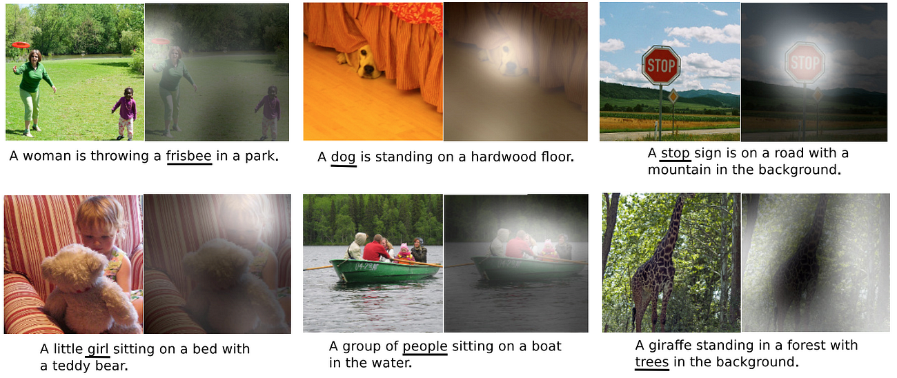
Figure 6: Attending to objects in an image during caption generation. The white regions indicate where the attention mechanism focused on during the generation of the underlined word. From Xu, Kelvin, et al. “Show, attend and tell: Neural image caption generation with visual attention.” International Conference on Machine Learning. 2015.
The creators of SpaCy have an in-depth overview of the encoder-attention-decoder paradigm. For other ways of modifying RNNs you can head over to this Distill article.
This tutorial will feature a single bidirectional LSTM as the encoder and the attention decoder (more on this later). More concretely, we will implement a simpler version of the model presented in “Neural machine translation by jointly learning to align and translate.” (Bahdanau, Dzmitry, Kyunghyun Cho, and Yoshua Bengio.2014). I’ll walk through some of the math, but I invite you to jump into the appendices of the paper to get your hands dirty!
Now that we have learned about RNNs and the intuition behind the attention mechanism, let us learn how to implement it and subsequently obtain some nice visualizations. All code for subsequent sections is provided at datalogue/keras-attention. The complete implementation of the model below is in /models/NMT.py
The Encoder
Since we are trying to learn about AttentionRNNs, we will skip implementing our own vanilla RNN (LSTM) and use the one that ships with Keras. We can invoke it using:
BLSTM = Bidirectional(LSTM(encoder_units, return_sequences=True))
The parameter encoder_units is the size of the weight matrix. We use return_sequences=True here because we'd like to access the complete encoded sequence rather than the final summary state as described above.
Our BLSTM will consume the charactersin the input sentence x=(x1,...,xT)and output an encoded sequence h=(h1,...,hT) where T is the number of characters in the date. Note that this is slightly different to the Bahdanau et al. paper where the sentence is a collection of words rather than characters. We also do not refer to the encoded sequence as the annotationslike in the original paper.
The Decoder
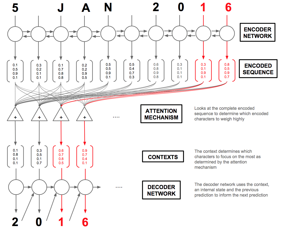
Figure 7: Overview of the Attention mechanism in an Encoder-Decoder setup.The attention mechanism creates context vectors. The decoder network uses these context vectors as well as the previous prediction to make the next one. The red arrows highlight which characters the attention mechanism will weigh highly in producing the output characters “1” and “6”.
Now for the interesting part: the decoder. For any given character at position t in the sequence, our decoder accepts the encoded sequence h=(h1,...,hT)as well as the previous hidden state st-1(shared within the decoder cell) and character yt-1. Our decoder layer will output y=(y1,...,yT)(the characters in the standardized date). Our overall architecture is summarized in Figure 7.
Equations
As shown in Figure 6, the decoder is quite complicated. So let’s break it down into the steps executed by the decoder cell when trying to predict character t.In the following equations, the capital letter variables represent trainable parameters (Note that I have dropped the bias terms for brevity.)

Equation 1:A feed-forward neural network that calculates the unnormalized importance of character j in predicting character t. Equation 2: The softmaxoperation that normalizes the probability.
- Calculate the attention probabilities
α=(α1,…,αT)based on the encoded sequence and the internal hidden state of the decoder cell,st-1.These are shown in Equation 1 and Equation 2.

Figure 3:Calculation of the context vector for the t-th character.
2. Calculate the contextvector which is the weighted sum of the encoded sequence with the attention probabilities. Intuitively, this vector summarizes the importance of the different encoded characters in predicting the t-th character.

Equation 4:Reset gate. Equation 5: Update gate. Equation 6:Proposal hidden state. Equation 7:New hidden state.
3. We then update our hidden state. If you are familiar with the equations of an LSTM cell, these might be ring a bell as the reset gate, r, update gate, z, and the proposal state. We use the reset gate to control how much information from the previous hidden state st-1is used to create a proposal hidden state. The update gate controls how we much of the proposal we use in the new hidden state st. (Confused? See step by step walk through of LSTM equations)

Equation 8: A simple neural network to predict the next character.
4. Calculate the t-th character using a simple one layer neural network using the context, hidden state, and previous character. This is a modification from the paper which uses a maxout layer. Since we are trying to keep things as simple as possible this works fine!
Equations 1–8 are applied for every character in the encoded sequence to produce a decoded sequence y which represents the probability of a translated character at each position.
Code
Our custom layer is implemented in models/custom_recurrent.py. This part is somewhat complicated in particular because of the manipulations we need to make for vectorized operations acting on the complete encoded sequence. It will make more sense when you think about it. I promise it will become easier the more you look at the equations and the code simultaneously.
A minimal custom Keras layer has to implement a few methods: __init__, compute_ouput_shape, build and call. For completeness, we also implement get_config which allows you to load the model back into memory easily. In addition to these, a Keras recurrent layer implements a step method that will hold all the computations of our cell.
First let us break down boiler-plate layer code:
__init__is what is called when the Layer is first instantiated. It sets functions that will eventually initialize the weights, regularizers, and constraints. Since the output of our layer is a sequence, we hard codeself.return_sequences=True.buildis called when we runModel.compile(…). Since our model is quite complicated, you can see there are a ton of weights to initialize here. The callself.add_weightautomatically handles initializing the weights and setting them as trainable within the model. Weights with the subscriptaare used to calculate the context vector (step 1 and 2). Weights with the subscriptr,z,pwill calculate the new hidden states from step 3. Finally, weights with the subscriptowill calculate the output of the layer.- Some convenience functions are implemented as well: (a)
compute_output_shapewill calculate output shapes for any given input; (b)get_configlet’s us load the model using just a saved file (once we are done training)
Now for the cell logic:
- By default, each execution of the cell only has information from the previous time step. Since we need to access the entire encoded sequence within the cell, we need to save it somewhere. Therefore, we make a simple modification in
call. The only way I could find to do this was to set the sequence being fed into the cell asself.xso that we can access it later:
Now we need to think vectorized: The _time_distributed_dense function calculates the last term of Equation 1 for all the elements of the encoded sequence.
- We now walk through the most important part of the code, that is in
stepwhich executes the cell logic. Recall thatstepis applied to every element of the input sequence.
In this cell we want to access the previous character ytm and hidden state stm which is obtained from states in line 4.
Think vectorized: we manipulate stm to repeat it for the number of characters we have in our input sequence.
On lines 11–18 we implement a version of equation 1 that does the calculations on all the characters in the sequence at once.
In lines 24–28 we have implemented Equation 2 in the vectorized form for the whole sequence. We use repeat to allow us to divide every time step by the respective sums.
To calculate the context vector, we need to keep in mind that self.x_seq and at have a “batch dimension” and therefore we need to use batch_dot to avoid doing the multiplication over that dimension. The squeeze operation just removes left-over dimensions. This is done in lines 33–37.
The next few lines of code are a more straightforward implementation of equations 4 –8.
Now we think a bit ahead: We would like to calculate those fancy attention maps in Figure 1. To do this, we need a “toggle” that returns the attention probabilities at.
Training
Data
Any good learning problem should have training data. In this case, it’s easy enough thanks to the Faker library which can generate fake dates with ease. I also use the Babel library to generate dates in different languages and formats as inspired by rasmusbergpalm/normalization. The script data/generate.py will generate some fake data and I won’t bore you with the details but invite you to poke around or to make it better.
The script also generates a vocabulary that will convert characters into integers so that the neural network can understand it. Also included is a script in data/reader.py to read and prepare data for the neural network to consume.
Model
This simple model with a bidirectional LSTM and the decoder we wrote above is implemented in models/NMT.py. You can run it using python run.py where I have set some default arguments (Readme has more information). I’d recommend training on a machine with a GPU as it can be prohibitively slow on a CPU-only machine.
If you want to skip the training part, I have provided some weights in weights/
Visualization
Now the easy part. For the visualizer implemented in visualizer.py, we need to load the weights in twice: Once with the predictive model, and the other to obtain the probabilities. Since we implemented the model architecture in models/NMT.py we can simply call the function twice:
from models.NMT import simpleNMT
predictive_model = simpleNMT(...)
predictive_model.load_weights(..., return_probabilities=False)
probability_model = simpleNMT(..., return_probabilities=True)
probability_model.load_weights(...)
To simply use the implemented visualizer, you can type:
python visualizer.py -h
to see available command line arguments.
Example visualizations
Let us now examine the attentions we generated from probability_model. The predictive_model above returns the translated date that you see on the y-axis. On the x-axis is our input date. The map shows us which input characters (on the x-axis) were used in the prediction of the output character on the y-axis. The brighter the white, the more weight that character had. Here are some I thought were quite interesting.
A correct example which doesn’t pay attention to unnecessary information like days of the week:
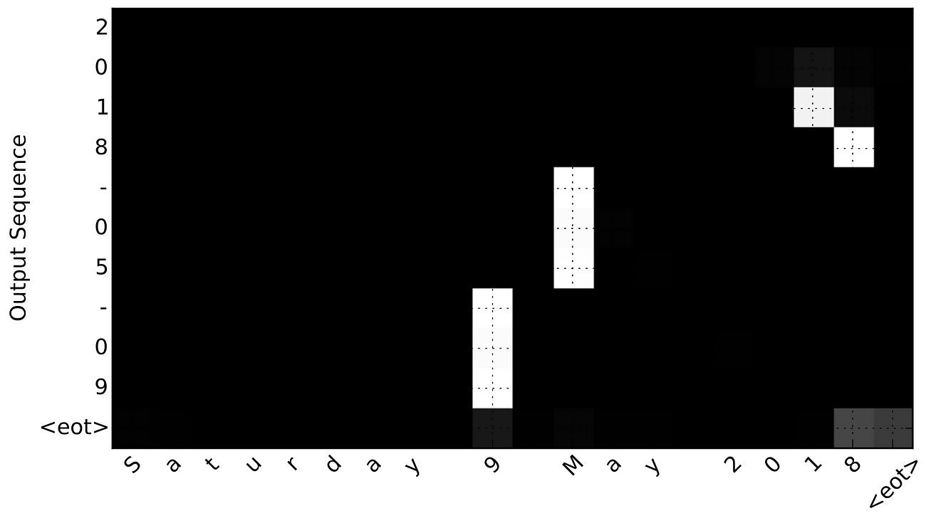
Example 1:The model has learned to ignore “Saturday” during translation. We can observe that “9” is used in the prediction of “-09” (the day). The letter “M” is used to predict “-05” (the month). The last two digits of 2018 are used to predict the year.
And here is an example of an incorrect translation because we submitted our example text in a novel order: “January 2016 05” was translated to “2016–01–02” rather than “2016–01–05”.
We can see that the model has mistakenly interpreted the characters “20” from 2016 as the day of the month. The activations are weak (some even correctly on the actual date of “5”) which can provide us with some insight into how to better train this model.
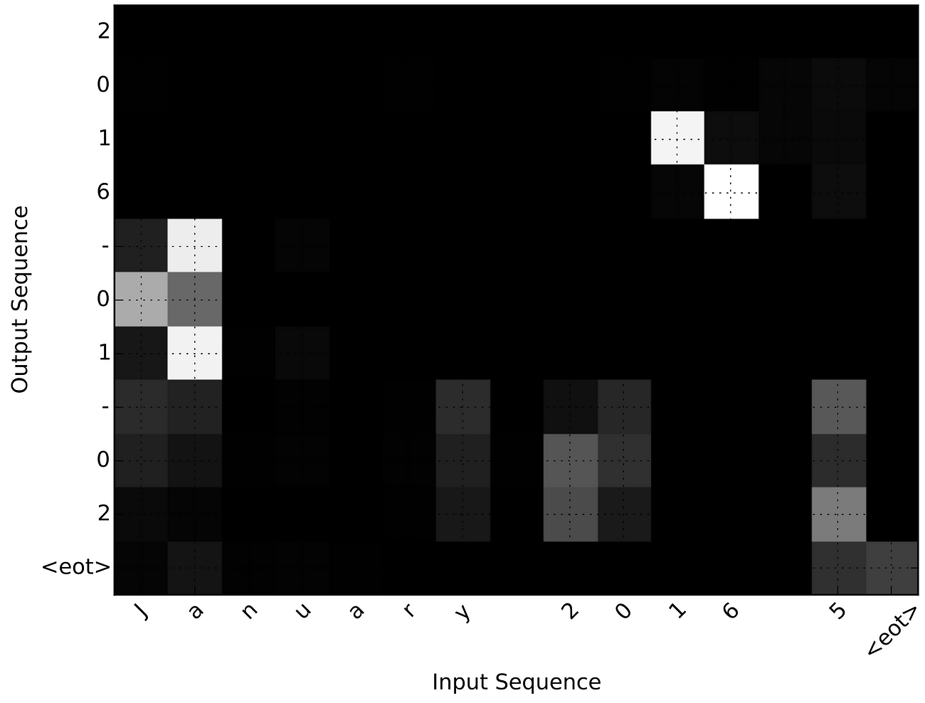
Example 2:We can see the weirdly formatted date “January 2016 5” is incorrectly translated as 2016–01–02 where the “02” comes from the “20” in 2016
Conclusion
I hope this tutorial has shown you how to solve a machine learning problem from start to finish. Furthermore, I hope it helps you in trying to visualize seq2seq problems with recurrent neural networks. If there is something I missed or you think I could do better, please feel free to reach out via twitter or make an issue on our github, I’d love to chat!
Acknowledgements
Zaf is an intern at Datalogue partially supported by an NSERC Experience Award. The Datalogue Team contributed for code review and reading the proofs of this post.
原文地址: https://medium.com/datalogue/attention-in-keras-1892773a4f22
How to Visualize Your Recurrent Neural Network with Attention in Keras相关推荐
- (zhuan) Recurrent Neural Network
Recurrent Neural Network 2016年07月01日 Deep learning Deep learning 字数:24235 this blog from: http://jxg ...
- Recurrent Neural Network系列2--利用Python,Theano实现RNN
作者:zhbzz2007 出处:http://www.cnblogs.com/zhbzz2007 欢迎转载,也请保留这段声明.谢谢! 本文翻译自 RECURRENT NEURAL NETWORKS T ...
- 深度学习之递归神经网络(Recurrent Neural Network,RNN)
为什么有bp神经网络.CNN.还需要RNN? BP神经网络和CNN的输入输出都是互相独立的:但是实际应用中有些场景输出内容和之前的内 容是有关联的. RNN引入"记忆"的概念:递归 ...
- 论文学习15-Table Filling Multi-Task Recurrent Neural Network(联合实体关系抽取模型)
文章目录 abstract 1 introduction 2.方 法 2.1实体关系表(Figure-2) 2.2 The Table Filling Multi-Task RNN Model 2.3 ...
- Recurrent Neural Network系列1--RNN(循环神经网络)概述
作者:zhbzz2007 出处:http://www.cnblogs.com/zhbzz2007 欢迎转载,也请保留这段声明.谢谢! 本文翻译自 RECURRENT NEURAL NETWORKS T ...
- 【李宏毅机器学习】Recurrent Neural Network Part1 循环神经网络(p20) 学习笔记
李宏毅机器学习学习笔记汇总 课程链接 文章目录 Example Application Slot Filling 把词用向量来表示的方法 1-of-N encoding / one-hot Beyon ...
- 2021李宏毅机器学习课程笔记——Recurrent Neural Network
注:这个是笔者用于期末复习的一个简单笔记,因此难以做到全面详细,有疑问欢迎大家在评论区讨论 I. Basic Idea 首先引入一个例子,槽填充(Slot Filling)问题: Input: I w ...
- Quasi Recurrent Neural Network (QRNNs) (git待更新...)
文章目录 1. Introduction 2.模型详解 2.1. 卷积 2.2. 池化 相关代码 参考文献 工程化的时候总会考虑到性能和效率,今天的主角也是基于这个根源,最终目的是在准确率保证的前提下 ...
- Attention-Based Recurrent Neural Network Models for Joint Intent Detection and Slot Filling论文笔记
文章目录 摘要 方法 Encoder-Decoder Model with Aligned Inputs Attention-Based RNN Model 实验 论文连接:Attention-Bas ...
最新文章
- Spring JdbcTemplate小结
- 源路由 就是指定数据传输经过这个路由服务器
- MySQL——高阶语句、存储过程(下)
- eclipse创建pojo_使用Eclipse Hibernate插件逐步为POJO域Java类和hbm自动生成代码
- Java泛型中extends和super的区别?
- linux 创建进程 execl,linux中进程的vfork()和execl()函数
- Atititi. naming spec 联系人命名与remark备注指南规范v5 r99.docx
- 使用油猴插件,屏蔽网页上的禁止右键操作
- Airtag小贵但好用?Beacon防丢功能体验
- win10开始菜单点击无效(win10开始菜单点击无效,网络不启动,音频不启动)
- jdk卸载,提示Windows Installer安装包有问题,此程序所需要的dll不能运行
- 蔡学镛[散文随笔]:从A到E+
- Delphi @ ^
- matlab stem函数坐标轴_在MATLAB中可以设置坐标轴的函数详解
- .split()用法解释
- 【Python黑科技】获取每日一句美句,并定时发送邮件到指定邮箱(保姆级图文+实现代码)
- 【STM32H7】第4章 ThreadX FileX文件系统移植到STM32H7(SD卡)
- 必应每日壁纸图片API
- 智能合约审计之访问控制
- 简述改变计算机桌面背景的方法,桌面背景不能更换怎么办 桌面背景不能更换解决方法【详细介绍】...