立即学习AI (Learn AI Today)

This is the first story in the Learn AI Today series I’m creating! These stories, or at least the first few, are based on a series of Jupyter notebooks I’ve created while studying/learning PyTorch and Deep Learning. I hope you find them as useful as I did!

这是《 今日学习AI》中的第一个故事 我正在创建的系列！ 这些故事，或者至少是前几篇小说，是基于我在学习/学习PyTorch和Deep Learning时创建的一系列Jupyter笔记本的 。 希望您发现它们和我一样有用！

您将从这个故事中学到什么： (What you will learn in this story:)

• How to Create a PyTorch Model如何创建PyTorch模型
• How to Train Your Model如何训练模型
• Visualize the Training Progress Dynamically动态可视化培训进度
• How the Learning Rate Affects the Training学习率如何影响培训

1. PyTorch中的线性回归 (1. Linear Regression in PyTorch)

Linear regression is a problem that you are probably familiar with. In it’s most basic form is no more than fitting a line to a set of points.

线性回归是您可能熟悉的问题。 最基本的形式就是将一条直线拟合到一组点。

1. 1概念介绍 (1. 1 Introducing the Concepts)

Consider the mathematical expression of a line:

考虑一条线的数学表达式：

w and bare the two parameters or weights of this linear model. In machine learning, it is common to use w referring to weights and b referring to the bias parameter.

w和b是此线性模型的两个参数或权重 。 在机器学习中 ，通常使用w表示权重 ， b表示偏差参数。

In machine learning when we are training a model we are basically finding the optimal parameters w and b for a given set of input/target (x,y) pairs. After the model is trained we can compute the model estimates. The expression will now look

在机器学习中，当我们训练模型时 ，基本上是为给定的一组输入/目标(x,y)对找到最佳参数 w和b 。 训练模型后，我们可以计算模型估计值。 表达式现在看起来

where I change the name o y to ye (y estimate) because the solution will not be exact.

在这里我将名称y更改为ye (y估计)，因为解决方案将不准确。

The Mean Square Error (MSE) is simply mean((ye-y)²) — the mean of the squared deviations between targets and estimates. For a regression problem, you can indeed minimize the MSE in order to find the best w and b .

均方误差(MSE)就是mean((ye-y)²) -目标与估算值之间平方差的均值。 对于回归问题，您确实可以最小化MSE以便找到最佳的w和b 。

The idea of linear regression can be generalized using algebra matrix notation to allow for multiple inputs and targets. If you want to learn more about the mathematical exact solution for the regression problem you can search about Normal Equation.

线性回归的思想可以使用代数矩阵符号来概括，以允许多个输入和目标。 如果您想了解有关回归问题的数学精确解的更多信息，可以搜索正态方程 。

1.2定义模型 (1.2 Defining the Model)

PyTorch nn.Linear class is all that you need to define a linear model with any number of inputs and outputs. For our basic example of fitting a line to a set of points consider the following model:

PyTorch nn.Linear类是定义具有任意数量的输入和输出的线性模型所需的全部。 对于将线拟合到一组点的基本示例，请考虑以下模型：

Note: I’m using Module from fastai library as it makes the code cleaner. If you want to use pure PyTorch you should use nn.Module instead and you need to add super().__init__() in the __init__ method. fastai Module does that for you.

注意： 我正在使用 来自 fastai 库的 Module ， 因为它使代码更 简洁 。 如果要使用纯PyTorch，则应改用 nn.Module 并且需要 在 __init__ 方法中 添加 super().__init__() 。 fastai Module 为您做到这一点。

If you are familiar with Python classes, the code is self-explanatory. If not, consider doing some study before diving into PyTorch. There are many online tutorials and lessons covering the topic.

如果您熟悉Python类 ，则代码是不言自明的。 如果没有，请考虑在进入PyTorch之前进行一些研究。 有很多有关该主题的在线教程和课程。

Back to the code. In the __init__ method, you define the layers of the model. In this case, it is just one linear layer. Then, the forward method is the one that is called when you call the model. Similar to __call__ method in normal Python classes.

回到代码。 在__init__方法中，定义模型的层。 在这种情况下，它只是一个线性层。 然后， forward方法是调用模型时调用的方法。 与普通Python类中的__call__方法相似。

Now you can define an instance of your LinearRegression model as model = LinearRegression(1, 1) indicating the number of inputs and outputs.

现在，您可以将LinearRegression模型的实例定义为model = LinearRegression(1, 1)指示输入和输出的数量。

Maybe you are now asking why I don’t simply do model = nn.Linear(1, 1) and you are absolutely right. The reason I’m having all the trouble of defining LinearRegression class is just to work as a template for future improvements as you will find later.

也许您现在在问为什么我不只是简单地执行model = nn.Linear(1, 1)而您绝对正确。 我在定义LinearRegression类时遇到了LinearRegression麻烦，其LinearRegression只是为了用作将来改进的模板，您将在以后发现。

1.3如何训练模型 (1.3 How to Train Your Model)

The training process is based on a sequence of 4 steps that repeat iteratively:

培训过程基于4个步骤的序列，这些步骤可以重复进行：

• Forward pass: The input data is given to the model and the model outputs are obtained — outputs = model(inputs)

  正向传递：将输入数据提供给模型，并获得模型输出- outputs = model(inputs)

• The loss function is computed: For the purpose of the linear regression problem, the loss function we are using is the mean squared error (MSE). We often refer to this function as the criterion — loss = criterion(outputs, targets)

  计算损失函数：就线性回归问题而言，我们使用的损失函数为均方误差(MSE)。 我们通常将此函数称为准则- loss = criterion(outputs, targets)

• Backward pass: The gradients of the loss function with respect to each learnable parameter are computed. Remember that we want to reduce the loss function to make the outputs close to the targets. The gradients tell how the loss change if you increase or decrease each parameter — loss.backwards()

  向后传递：计算损失函数相对于每个可学习参数的梯度。 请记住，我们要减少损失函数以使输出接近目标。 梯度表明如果增加或减少每个参数，损失将如何变化— loss.backwards()

• Update parameters: Update the value of the parameters by a small amount in the direction that reduces the loss. The method to update the parameters can be as simple as subtracting the value of the gradient multiplied by a small number. This number is referred to as the learning rate and the optimizer I just described is the Stochastic Gradient Descent (SGD) — optimizer.step()

  更新参数：在减少损耗的方向上少量更新参数值。 更新参数的方法可以很简单，只要减去梯度值乘以一个小数即可。 该数字称为学习率 ，我刚才描述的优化器是随机梯度下降(SGD) — optimizer.step()

I didn’t define exactly the criterion and optimizer yet but I will in a minute. This is just to give you a general overview and understanding of the steps for a training iteration or as usually called — a training epoch.

我尚未确切定义criterion和optimizer ，但我会在一分钟内完成。 这只是为了使您对培训迭代的步骤或通常称为培训纪元的步骤有一个大致的了解。

Let’s define our fit function that will do all the required steps.

让我们定义执行所有必需步骤的fit函数。

Notice that there’s an extra step I didn’t mention before — optimizer.zero_grad() . This is because by default, in PyTorch, when you call loss.backwards() the optimizer adds up the values of the gradients. If you don’t set them to zero at each epoch then they will be always added up and that’s not desirable. Unless you are doing gradient accumulation — but that’s a more advanced topic. Besides that, as you can see in the code above, I’m saving the value of the loss at each epoch. We should expect it to drop steadily — meaning that the model is getting better at predicting the targets.

请注意，还有一个我之前没有提到的额外步骤 optimizer.zero_grad() 。 这是因为默认情况下，在PyTorch中，当您调用loss.backwards() ，优化器会累加渐变的值。 如果您没有在每个时期将它们设置为零，那么它们将总是相加，这是不希望的。 除非您要进行梯度累积，否则这是一个更高级的主题。 除此之外，如您在上面的代码中看到的那样，我保存了每个时期的损失值。 我们应该期望它会稳定下降-这意味着该模型在预测目标方面会变得更好。

As I mentioned above, for linear regression the criterion usually used is the MSE. As for the optimizer, nowadays I always use Adam as my first choice. It’s fast and it should work well for most problems. I won’t go into details about how Adam works for now but the idea is always to find the best solution in the least amount of time.

如上所述，对于线性回归，通常使用的标准是MSE 。 至于优化器，如今，我始终以Adam为首选。 它的速度很快，并且对于大多数问题都应该很好用。 我现在不会详细介绍Adam的工作方式，但该想法始终是在最短的时间内找到最佳解决方案。

Let’s now move on to creating an instance of our LinearRegression model, defining our criterion and our optimizer:

现在，让我们继续创建LinearRegression模型的实例，定义我们的标准和优化器 ：

model.parameters() is the way to give the optimizer the list of trainable parameters and lr is the learning rate.

model.parameters()是为优化器提供可训练参数列表的方法，而lr是学习率。

Now let’s create some data and train the model!

现在，让我们创建一些数据并训练模型！

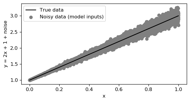
The data is simply a set of points following the model y = 2x + 1 + noise. To make it a little more interesting I make the noise larger for larger values of x. The unsqueeze(-1) in lines 4 and 5 is just to add an extra dimension to the tensor at the end (from [10000] to [10000,1] ). The data is the same but the tensor needs to have this shape meaning that we have 10000 samples and 1 feature per sample.

数据只是遵循模型y = 2x + 1 + noise一组点。 为了使它更有趣，我针对较大的x值使噪声更大。 第4行和第5行中的unsqueeze(-1)只是在末端的张量上添加了一个额外的维度(从[10000]到[10000,1] )。 数据是相同的，但张量必须具有此形状，这意味着我们有10000个样本，每个样本1个特征。

Plotting the data, the result is the image below, where you can see the true model and the input data + noise.

绘制数据，结果是下面的图像，您可以在其中看到真实的模型和输入数据+噪声。

And now to train the model we just run our fit function!

现在要训练模型，我们只需运行我们的 fit 函数！

After training, we can plot the evolution of the loss during the 100 epochs. As you can see in the image below, initially the loss was of about 2.0 and then it drops steeply down to nearly zero. This is to be expected since when we start the model parameters are randomly initialized and as the training progress they converge to the solution.

训练后，我们可以绘制出100个时期内损耗的演变图。 如下图所示，最初的损失约为2.0，然后急剧下降至接近零。 这是可以预期的，因为当我们开始时，模型参数是随机初始化的，并且随着训练的进行，它们收敛到解。

Note: Try playing with the learning rate value to see how it affects the training!

注意：尝试使用学习率值来查看它如何影响训练！

To check the parameters of the trained model, you can run list(model.parameters()) after training the model. You will see that they are very close to 2.0 and 1.0 for this example since the true model is y = 2x + 1 .

要检查已训练模型的参数，可以在训练模型后运行list(model.parameters()) 。 在本例中，您将看到它们非常接近2.0和1.0，因为真实模型为y = 2x + 1 。

You can now compute the model estimates — ye = model(x_train). (Notice that before computing the estimates you should always run model.eval() to set the model to evaluation mode. It won’t make a difference for this simple model but later it will, when we start using Batch Normalization and Dropout.)

您现在可以计算模型估计值ye = model(x_train) 。 (请注意，在计算估算值之前，应始终运行model.eval()将模型设置为评估模式。对于此简单模型而言，这没有什么不同，但是稍后，当我们开始使用批标准化和Dropout时，它将有所不同。)

Plotting the prediction you can see that it matches almost perfectly the true data, despite the fact that the model could only see the noisy data.

通过绘制预测，您可以看到它几乎与真实数据完全匹配，尽管该模型只能看到嘈杂的数据。

2.逐步进行多项式回归 (2. Stepping Up to Polynomial Regression)

Now that we made it work for the simple case, moving to a more complex linear model is remarkably simple. The first step is of course to generate such input data. For this example, I considered the model y = 3x² + 2x + 1 + noise as follows:

现在我们使它适用于简单的情况，转移到更复杂的线性模型非常简单。 第一步当然是生成此类输入数据。 对于此示例，我认为模型y = 3x² + 2x + 1 + noise如下：

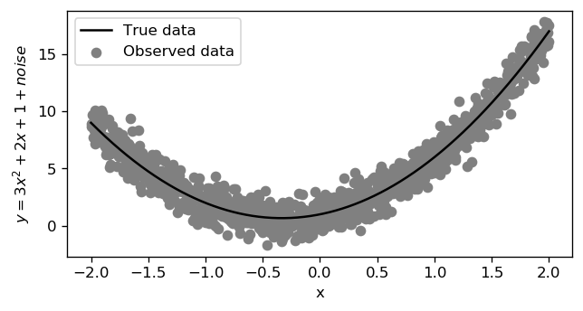
Notice that this time the input shape is [1000, 2] since we have 2 features corresponding to x and x² . That’s how you fit a polynomial using linear regression!

请注意，这一次输入形状为[1000, 2]因为我们有2个对应于x和x² 。 这就是使用线性回归拟合多项式的方式！

The only difference now, compared to the previous example, is that the model needs to have two inputs — model = LinearRegression(2,1) . That’s it! You can now follow the exact same steps to train the model.

与前一个示例相比，现在唯一的区别是该模型需要具有两个输入model = LinearRegression(2,1) 。 而已！ 现在，您可以按照完全相同的步骤来训练模型。

Let’s, however, make things a little more fun with some dynamical visualizations!

但是，让我们通过一些动态可视化使事情变得更加有趣！

2.1动态可视化培训进度 (2.1 Visualize the Training Progress Dynamically)

To animate the evolution of training we need to update the fit function in order to store also the values of the model estimates at each step.

为了动画化训练的演变，我们需要更新拟合函数，以便在每个步骤还存储模型估计值。

You may have noticed a ‘new word’ — detach() (line 17 of the code). This is to tell PyTorch to detach the variable from the gradient computation graph (it will no longer compute the gradients for that detached variable). If you try to convert the tensor to NumPy before detaching, it will give you an error.

您可能已经注意到一个“新词” — detach() (代码的第17行)。 这是告诉PyTorch从梯度计算图中分离变量(它将不再计算该分离变量的梯度)。 如果尝试在分离前将张量转换为NumPy，它将给您一个错误。

Moving on, you can repeat the same process to train the model as before. The only difference is that the fit2 function will also return the model estimates for each epoch of training.

继续，您可以像以前一样重复相同的过程来训练模型。 唯一的区别是fit2函数还将为每个训练时期返回模型估计。

To create a video/gif of the training take a look at the following code:

要创建培训的视频/ gif，请看以下代码：

The %%capture tells Jupyter to suppress the output of the cell as we will be displaying the video in the next cell. Then, from lines 3 to 10, I set up the plot as usual. The difference is in the line for the model predictions. I initiate it as empty to then iteratively update the graphic using matplotlib.animation to generate the animation. Finally, the video can be rendered using HTML from IPython.display . Look at the result below!

%%capture告诉Jupyter抑制单元格的输出，因为我们将在下一个单元格中显示视频。 然后，从第3行到第10行，照常设置图表。 区别在于模型预测。 我将其初始化为空，然后使用matplotlib.animation迭代更新图形以生成动画。 最后，可以使用IPython.display HTML渲染视频。 看下面的结果！

It’s interesting that the blue line initially curves very fast to the correct shape and then converges more slowly for the final solution!

有趣的是，蓝线最初会非常快地弯曲到正确的形状，然后会慢慢收敛以得到最终解决方案！

Note: Try playing with the learning rate, different optimizer and anything you can think off and see the effect on the optimization. It’s a good way to get some intuition for how the optimization works!

注意：尝试使用学习率 ，其他优化程序以及您可以考虑的所有内容，并查看对优化的影响。 这是了解优化工作原理的好方法！

3.神经网络模型 (3. Neural Network Model)

The examples above are interesting for learning and experimenting. However, in practice often your data is not generated from a polynomial or at least you don’t know what the terms of the polynomial are. A nice thing about neural networks is that you don’t need to worry about it!

上面的示例对于学习和实验很有趣。 但是，实际上，您的数据通常不是从多项式生成的，或者至少您不知道多项式的项是什么。 关于神经网络的一件好事是，您不必担心它！

Let’s start by defining the model that I named as GeneralFit :

首先定义我命名为GeneralFit的模型：

There are some new aspects to consider in this model. There are 3 linear layers and as you can see in the forward method, after the first two linear layers a ReLU activation function — F.relu() — is used. ReLU stands for Rectified Linear Unit and it’s simply setting all negatives to zero. This apparently trivial operation is, however, enough to make the model non-linear.

此模型中需要考虑一些新方面。 有3个线性层，正如您在正向方法中所看到的，在前两个线性层之后，使用了ReLU 激活函数 F.relu() 。 ReLU代表“ 整流线性单位” ，它只是将所有负数设置为零 。 但是，这种看似微不足道的操作足以使模型非线性。

Notice that a Linear layer is just matrix multiplication. If you have 100 linear layers one after the other, linear algebra tells you that there’s a single linear layer that performs the same operation. That single linear layer is simply the multiplication of the 100 matrices. However, when you introduce the non-linear activation function this changes completely. Now you can keep adding more linear layers interlaced with non-linear activations such as ReLU (most common in recent models).

注意，线性层只是矩阵乘法。 如果您有一个接一个的线性层，则线性代数会告诉您只有一个线性层执行相同的操作。 单个线性层就是100个矩阵的乘积。 但是，当您引入非线性激活函数时，它会完全改变。 现在，您可以继续添加更多与非线性激活(例如ReLU(在最近的模型中最常见))交织的线性层。

A Deep Neural Network is no more than a Neural Network with several ‘hidden’ layers. Looking back to the code above, you can, for example, try to add more ‘hidden’ layers and train the model. And indeed, you can call that Deep Learning. (Note that hidden layer is just the traditional name for any layers in between the input and output layer.)

深度神经网络只不过是具有多个“隐藏”层的神经网络。 回顾上面的代码，例如，您可以尝试添加更多的“隐藏”层并训练模型。 实际上，您可以将其称为“ 深度学习” 。 (请注意，隐藏层只是输入和输出层之间任何层的传统名称。)

Using the above model and a new set of generated data I obtained the following training animation:

使用以上模型和一组新的生成数据，我获得了以下训练动画：

For this example, I trained for 200 epochs with a learning rate of 0.01. Let’s try to set the learning rate to 1.

在此示例中，我训练了200个时期，学习率为0.01。 让我们尝试将学习率设置为1。

Clearly this is not good! When the learning rate is too high the model may not converge properly to a good solution or may even diverge. If you set the learning rate to 10 or 100 it won’t go anywhere.

显然这不好！ 当学习率太高时 ，模型可能无法正确收敛到一个好的解决方案，甚至可能会发散。 如果您将学习率设置为10或100，它将不会起作用。

家庭作业 (Homework)

I can show you a thousand examples but you will learn more if you can make one or two experiments by yourself! The complete code for these experiments that I showed you are available on this notebook.

我可以为您展示一千个示例，但是如果您可以自己进行一两个实验，您会学到更多！ 我在笔记本上可以找到我为您展示的这些实验的完整代码。

• Try to play with the learning rate, number of epochs, number of hidden layers and the size of the hidden layers;

  尝试发挥学习率 ，时期数，隐藏层数和隐藏层的大小；

• Try also SGD optimizer and play with the learning rate and maybe also with the momentum (I didn’t cover it in this story but now that you know about it you can do some research);也可以尝试使用SGD优化器，并利用学习率和动力(我没有在本故事中介绍它，但是现在您知道了，可以进行一些研究)；

If you create interesting notebooks with nice animations as a result of your experiments, go ahead and share it on GitHub, Kaggle or write a Medium story about it!

如果您通过实验创建了带有漂亮动画的有趣笔记本，请继续在GitHub，Kaggle上共享它，或撰写有关它的中型故事！

结束语 (Final remarks)

This ends the first story in the Learn AI Today series!

到此为止，《今日学习AI》系列的第一个故事！

• Please consider joining my mailing list in this link to get updates so that you won’t miss any of the following stories or important updates!

  请考虑通过此链接加入我的邮件列表 获取更新，这样您就不会错过以下任何故事或重要更新！

• I will also be listing the new stories at learn-ai-today.com, the page I created for this learning journey!

  我还将在learning-ai-today.com上列出新故事，该页面是我为这次学习之旅而创建的页面！

• And if you missed it before, this is the link for the Kaggle notebook with the code for this story!

  而且，如果您之前错过了它，那么这是Kaggle笔记本的链接，其中包含此故事的代码 ！

Feel free to give me some feedback in the comments. What did you find most useful or what could be explained better? Let me know!

请随时在评论中给我一些反馈。 您觉得最有用的是什么？ 让我知道！

Next story in this series:

本系列的下一个故事：

You can read more about my journey on the following stories!

您可以在以下故事中阅读有关我的旅程的更多信息！

Thanks for reading! Have a great day!

谢谢阅读！ 祝你有美好的一天！