Python is a highly powerful general purpose programming language which can be easily learned and provides data scientists a wide variety of tools and packages. Amid this pandemic period, I decided to do an analysis on this novel coronavirus.

Python是一种功能强大的通用编程语言，可以轻松学习，并为数据科学家提供各种工具和软件包。 在这个大流行时期，我决定对这种新型冠状病毒进行分析。

In this article, I am going to walk you through the steps I undertook for this analysis with visuals and code snippets.

在本文中，我将通过视觉和代码片段逐步指导您进行此分析。

数据分析涉及的步骤： (Steps involved in Data Analysis:)

1. Importing required packages导入所需的软件包

2. Gathering Data

2.收集数据

3. Transforming Data to our needs (Data Wrangling)

3.将数据转变为我们的需求(数据整理)

4. Exploratory Data Analysis (EDA) and Visualization

4.探索性数据分析(EDA)和可视化

步骤— 1：导入所需的软件包 (Step — 1: Importing required Packages)

Importing our required packages is the starting point of all data analysis programming in python. As I’ve said, python provides a wide variety of packages for data scientists and in this analysis I used python’s most popular data science packages Pandas and NumPy for Data Wrangling and EDA. When coming to Data Visualization, I used python’s interactive packages Plotly and Matplotlib. It’s very simple to import packages in python code:

导入所需的软件包是python中所有数据分析编程的起点。 就像我说过的那样，python为数据科学家提供了各种各样的软件包，在此分析中，我使用了python最受欢迎的数据科学软件包Pandas和NumPy进行数据整理和EDA。 进行数据可视化时，我使用了python的交互式软件包Plotly和Matplotlib。 用python代码导入软件包非常简单：

This is the code for importing our primary packages to perform data analysis but still, we need to add some more packages to our code which we will see in step-2. Yay! We successfully finished our first step.

这是用于导入主要程序包以执行数据分析的代码，但是仍然需要向代码中添加更多程序包，我们将在步骤2中看到这些代码。 好极了！ 我们成功地完成了第一步。

步骤2：收集数据 (Step — 2: Gathering Data)

For a clean and perfect data analysis, the foremost important element is collecting quality Data. For this analysis, I’ve collected many data from various sources for better accuracy.

对于 干净，完美的数据分析，最重要的元素是收集高质量的数据。 为了进行此分析，我从各种来源收集了许多数据，以提高准确性。

Our primary dataset is extracted from esri (a website which provides updated data on coronavirus) using a query url (click here to view the website). Follow the code snippets to extract the data from esri:

我们的主要数据集是使用查询网址从esri(提供有关冠状病毒的最新数据的网站)中提取的( 请单击此处查看该网站 )。 按照代码片段从esri中提取数据：

Requests is a python packages used to extract data from a given json file. In this code I used requests to extract data from the given query url by esri. We are now ready to do some Data Wrangling! (Note : We will be importing many data in step-4 of our analysis)

Requests是一个python软件包，用于从给定的json文件中提取数据。 在这段代码中，我使用了esri的请求从给定的查询URL中提取数据。 现在，我们准备进行一些数据整理！ (注意：我们将在分析的第4步中导入许多数据)

步骤— 3：数据整理 (Step — 3: Data Wrangling)

Data Wrangling is a process where we will transform and clean our data to our needs. We can’t do analysis with our raw extracted data. So, we have to transform the data to proceed our analysis. Here’s the code for our Data Wrangling:

数据整理是一个过程，在此过程中，我们将根据需要转换和清理数据。 我们无法使用原始提取的数据进行分析。 因此，我们必须转换数据以进行分析。 这是我们的数据整理的代码：

Note that, we have imported a new python package, ‘datetime’, which helps us to work with dates and times in a dataset. Now, get ready to see the big picture of our analysis -’ EDA and Data Visualization’.

请注意，我们已经导入了一个新的python包“ datetime”，它可以帮助我们处理数据集中的日期和时间。 现在，准备看一下我们分析的大图-“ EDA和数据可视化”。

步骤— 4：探索性数据分析和数据可视化 (Step — 4: Exploratory Data Analysis and Data Visualization)

This process is quite long as it is the heart and soul of data analysis. So, I’ve divided this process into three steps:

这个过程很长，因为它是数据分析的心脏和灵魂。 因此，我将这一过程分为三个步骤：

a. Ranking countries and provinces (based on COVID-19 aspects)

一个。 对国家和省进行排名(基于COVID-19方面)

b. Time Series on COVID-19 Cases

b。 COVID-19病例的时间序列

c. Classification and Distribution of cases

C。 案件分类和分布

Ranking countries and provinces

排名国家和省

From our previously extracted data we are going to rank countries and provinces based on confirmed, deaths, recovered and active cases by doing some EDA and Visualization. Follow the code snippets for the upcoming visuals (Note : Every visualizations are interactive and you can hover them to see their data points)

从我们先前提取的数据中，我们将通过进行一些EDA和可视化，根据确诊，死亡，康复和活着的病例对国家和省进行排名。 请遵循即将出现的视觉效果的代码片段(注意：每个视觉效果都是交互式的，您可以将它们悬停以查看其数据点)

Part 1 — Ranking Most affected countries

第1部分-排名受影响最大的国家

i) Top 10 Confirmed Cases Countries:

i)十大确诊病例国家：

The following code will produce a plot ranking top 10 countries based on confirmed cases.

以下代码将根据已确认的案例得出前十个国家/地区的地块。

# a. Top 10 confirmed countries (Bubble plot)top10_confirmed = pd.DataFrame(data.groupby('Country')['Confirmed'].sum().nlargest(10).sort_values(ascending = False))
fig1 = px.scatter(top10_confirmed, x = top10_confirmed.index, y = 'Confirmed', size = 'Confirmed', size_max = 120,color = top10_confirmed.index, title = 'Top 10 Confirmed Cases Countries')
fig1.show()

演示地址

ii) Top 10 Death Cases Countries:

ii)十大死亡案例国家：

The following code will produce a plot ranking top 10 countries based on death cases.

以下代码将根据死亡案例产生一个排在前十个国家/地区的地块。

# b. Top 10 deaths countries (h-Bar plot)top10_deaths = pd.DataFrame(data.groupby('Country')['Deaths'].sum().nlargest(10).sort_values(ascending = True))
fig2 = px.bar(top10_deaths, x = 'Deaths', y = top10_deaths.index, height = 600, color = 'Deaths', orientation = 'h',color_continuous_scale = ['deepskyblue','red'], title = 'Top 10 Death Cases Countries')
fig2.show()

演示地址

iii) Top 10 Recovered Cases Countries:

iii)十大被追回病例国家：

The following code will produce a plot ranking top 10 countries based on recovered cases.

以下代码将根据恢复的案例生成一个排在前10个国家/地区的地块。

# c. Top 10 recovered countries (Bar plot)top10_recovered = pd.DataFrame(data.groupby('Country')['Recovered'].sum().nlargest(10).sort_values(ascending = False))
fig3 = px.bar(top10_recovered, x = top10_recovered.index, y = 'Recovered', height = 600, color = 'Recovered',title = 'Top 10 Recovered Cases Countries', color_continuous_scale = px.colors.sequential.Viridis)
fig3.show()

演示地址

iv) Top 10 Active Cases Countries:

iv)十大活跃案例国家：

The following code will produce a plot ranking top 10 countries based on recovered cases.

以下代码将根据恢复的案例生成一个排在前10个国家/地区的地块。

# d. Top 10 active countriestop10_active = pd.DataFrame(data.groupby('Country')['Active'].sum().nlargest(10).sort_values(ascending = True))
fig4 = px.bar(top10_active, x = 'Active', y = top10_active.index, height = 600, color = 'Active', orientation = 'h',color_continuous_scale = ['paleturquoise','blue'], title = 'Top 10 Active Cases Countries')
fig4.show()

演示地址

Part 2 — Ranking most affected States in largely affected Countries:

第2部分-在受影响最大的国家中对受影响最大的国家进行排名：

EDA for ranking states in largely affected Countries:

对受灾严重国家排名的EDA：

# USA
topstates_us = data['Country'] == 'US'
topstates_us = data[topstates_us].nlargest(5, 'Confirmed')
# Brazil
topstates_brazil = data['Country'] == 'Brazil'
topstates_brazil = data[topstates_brazil].nlargest(5, 'Confirmed')
# India
topstates_india = data['Country'] == 'India'
topstates_india = data[topstates_india].nlargest(5, 'Confirmed')
# Russia
topstates_russia = data['Country'] == 'Russia'
topstates_russia = data[topstates_russia].nlargest(5, 'Confirmed')

We are extracting States’ data from USA, Brazil, India and Russia respectively because, these are the countries which are most affected by COVID-19. Now, let’s visualize it!

我们分别从美国，巴西，印度和俄罗斯提取州的数据，因为这是受COVID-19影响最大的国家。 现在，让我们对其进行可视化！

Visualization of Most affected states in largely affected Countries:

受影响最大的国家中受影响最大的州的可视化：

i) Most affected States in USA:

i)美国受影响最严重的州：

The following code will produce a plot ranking top 5 most affected states in the United States of America.

以下代码将产生一个在美国受灾最严重的州中排名前5位的地块。

# USA
fig5 = go.Figure(data = [go.Bar(name = 'Active Cases', x = topstates_us['Active'], y = topstates_us['State'], orientation = 'h'),go.Bar(name = 'Death Cases', x = topstates_us['Deaths'], y = topstates_us['State'], orientation = 'h')
])
fig5.update_layout(title = 'Most Affected States in USA', height = 600)
fig5.show()

演示地址

ii) Most affected States in Brazil:

ii)巴西受影响最严重的国家：

The following code will produce a plot ranking top 5 most affected states in Brazil.

以下代码将产生一个在巴西受影响最严重的州中排名前5位的地块。

# Brazil
fig6 = go.Figure(data = [go.Bar(name = 'Recovered Cases', x = topstates_brazil['State'], y = topstates_brazil['Recovered']),go.Bar(name = 'Active Cases', x = topstates_brazil['State'], y = topstates_brazil['Active']),go.Bar(name = 'Death Cases', x = topstates_brazil['State'], y = topstates_brazil['Deaths'])
])
fig6.update_layout(title = 'Most Affected States in Brazil', barmode = 'stack', height = 600)
fig6.show()

演示地址

iii) Most affected States in India:

iii)印度受影响最大的国家：

The following code will produce a plot ranking top 5 most affected states in India.

以下代码将产生一个在印度受影响最严重的州中排名前5位的地块。

# India
fig7 = go.Figure(data = [go.Bar(name = 'Recovered Cases', x = topstates_india['State'], y = topstates_india['Recovered']),go.Bar(name = 'Active Cases', x = topstates_india['State'], y = topstates_india['Active']),go.Bar(name = 'Death Cases', x = topstates_india['State'], y = topstates_india['Deaths'])
])
fig7.update_layout(title = 'Most Affected States in India', barmode = 'stack', height = 600)
fig7.show()

演示地址

iv) Most affected States in Russia:

iv)俄罗斯受影响最严重的国家：

The following code will produce a plot ranking top 5 most affected states in Russia.

以下代码将产生一个在俄罗斯受影响最严重的州中排名前5位的地块。

# Russia
fig8 = go.Figure(data = [go.Bar(name = 'Recovered Cases', x = topstates_russia['State'], y = topstates_russia['Recovered']),go.Bar(name = 'Active Cases', x = topstates_russia['State'], y = topstates_russia['Active']),go.Bar(name = 'Death Cases', x = topstates_russia['State'], y = topstates_russia['Deaths'])
])
fig8.update_layout(title = 'Most Affected States in Russia', barmode = 'stack', height = 600)
fig8.show()

演示地址

Time Series on COVID-19 Cases

COVID-19病例的时间序列

To perform time series analysis on COVID-19 cases we need a new dataset. https://covid19.who.int/ Follow this link and images shown below for downloading our next dataset.

要对COVID-19案例执行时间序列分析，我们需要一个新的数据集。 https://covid19.who.int/请点击下面的链接和图像，下载我们的下一个数据集。

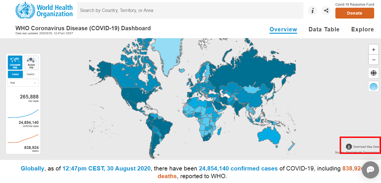
After pressing the link mentioned above, you will land into this page. On the bottom right of the represented map, you can find the download button. From there you can download the dataset and save it to your files. Good work! We fetched our Data! Let’s import the data :

按下上述链接后，您将进入此页面。 在所显示地图的右下角，您可以找到下载按钮。 从那里您可以下载数据集并将其保存到文件中。 干得好！ 我们获取了数据！ 让我们导入数据：

time_series = pd.read_csv('who_data.csv', encoding = 'ISO-8859-1')
time_series['Date_reported'] = pd.to_datetime(time_series['Date_reported'])

From the above extracted dataset, we are going to perform two types of time series analysis, ‘COVID-19 cases Worldwide’ and ‘Most affected countries over time’.

从上面提取的数据集中，我们将执行两种类型的时间序列分析：“全球COVID-19病例”和“一段时间内受影响最大的国家”。

i) COVID-19 cases worldwide:

i)全球COVID-19病例：

EDA for COVID-19 cases worldwide:

全球COVID-19案件的EDA：

time_series_dates = time_series.groupby('Date_reported').sum()
time_series_dates

a) Cumulative cases worldwide:

a)全世界的累积病例：

The following code produces a time series chart of cumulative cases worldwide right from the beginning of the outbreak.

以下代码从爆发开始就生成了全球累积病例的时序图。

# Cumulative casesfig11 = go.Figure()
fig11.add_trace(go.Scatter(x = time_series_dates.index, y = time_series_dates[' Cumulative_cases'], fill = 'tonexty',line_color = 'blue'))
fig11.update_layout(title = 'Cumulative Cases Worldwide')
fig11.show()

演示地址

b) Cumulative death cases worldwide:

b)世界范围内的累积死亡案例：

The following code produces a time series chart of cumulative death cases worldwide right from the beginning of the outbreak.

以下代码从爆发开始就生成了全球累积死亡病例的时间序列图。

# Cumulative death casesfig12 = go.Figure()
fig12.add_trace(go.Scatter(x = time_series_dates.index, y = time_series_dates[' Cumulative_deaths'], fill = 'tonexty',line_color = 'red'))
fig12.update_layout(title = 'Cumulative Deaths Worldwide')
fig12.show()

演示地址

c) Daily new cases worldwide:

c)全世界每天的新病例：

The following code produces a time series chart of daily new cases worldwide right from the beginning of the outbreak.

以下代码从爆发开始就生成了全球每日新病例的时序图。

# Daily new casesfig13 = go.Figure()
fig13.add_trace(go.Scatter(x = time_series_dates.index, y = time_series_dates[' New_cases'], fill = 'tonexty',line_color = 'gold'))
fig13.update_layout(title = 'Daily New Cases Worldwide')
fig13.show()

演示地址

d) Daily death cases worldwide:

d)全世界每日死亡案例：

The following code produces a time series chart of daily death cases worldwide right from the beginning of the outbreak.

以下代码从爆发开始就生成了全球每日死亡病例的时间序列图。

# Daily death casesfig14 = go.Figure()
fig14.add_trace(go.Scatter(x = time_series_dates.index, y = time_series_dates[' New_deaths'], fill = 'tonexty',line_color = 'hotpink'))
fig14.update_layout(title = 'Daily Death Cases Worldwide')
fig14.show()

演示地址

ii) Most affected countries over time:

ii)一段时间内受影响最大的国家：

EDA for Most affected countries over time:

随时间推移对受影响最严重国家的EDA：

# USA
time_series_us = time_series[' Country'] == ('United States of America')
time_series_us = time_series[time_series_us]# Brazil
time_series_brazil = time_series[' Country'] == ('Brazil')
time_series_brazil = time_series[time_series_brazil]# India
time_series_india = time_series[' Country'] == ('India')
time_series_india = time_series[time_series_india]# Russia
time_series_russia = time_series[' Country'] == ('Russia')
time_series_russia = time_series[time_series_russia]# Peru
time_series_peru = time_series[' Country'] == ('Peru')
time_series_peru = time_series[time_series_peru]

Note that, we have extracted data of countries USA, Brazil, India, Russia and Peru respectively as they are highly affected by COVID-19 in the world.

请注意，我们分别提取了美国，巴西，印度，俄罗斯和秘鲁等国家/地区的数据，因为它们在世界范围内受到COVID-19的高度影响。

a) Most affected Countries’ Cumulative cases over time

a)随时间推移受影响最严重的国家的累计案件

The following code will produce a time series chart of the most affected countries’ cumulative cases right from the beginning of the outbreak.

以下代码将从疫情爆发之初就产生受影响最严重国家累计病例的时序图。

# Cumulative casesfig15 = go.Figure()fig15.add_trace(go.Line(x = time_series_us['Date_reported'], y = time_series_us[' Cumulative_cases'], name = 'USA'))
fig15.add_trace(go.Line(x = time_series_brazil['Date_reported'], y = time_series_brazil[' Cumulative_cases'], name = 'Brazil'))
fig15.add_trace(go.Line(x = time_series_india['Date_reported'], y = time_series_india[' Cumulative_cases'], name = 'India'))
fig15.add_trace(go.Line(x = time_series_russia['Date_reported'], y = time_series_russia[' Cumulative_cases'], name = 'Russia'))
fig15.add_trace(go.Line(x = time_series_peru['Date_reported'], y = time_series_peru[' Cumulative_cases'], name = 'Peru'))fig15.update_layout(title = 'Time Series of Most Affected countries"s Cumulative Cases')fig15.show()

演示地址

b) Most affected Countries’ cumulative death cases over time:

b)随着时间的推移，大多数受影响国家的累计死亡病例：

The following code will produce a time series chart of the most affected countries’ cumulative death cases right from the beginning of the outbreak.

以下代码将从疫情爆发之初就绘制出受影响最严重国家累计死亡病例的时间序列图。

# Cumulative death casesfig16 = go.Figure()fig16.add_trace(go.Line(x = time_series_us['Date_reported'], y = time_series_us[' Cumulative_deaths'], name = 'USA'))
fig16.add_trace(go.Line(x = time_series_brazil['Date_reported'], y = time_series_brazil[' Cumulative_deaths'], name = 'Brazil'))
fig16.add_trace(go.Line(x = time_series_india['Date_reported'], y = time_series_india[' Cumulative_deaths'], name = 'India'))
fig16.add_trace(go.Line(x = time_series_russia['Date_reported'], y = time_series_russia[' Cumulative_deaths'], name = 'Russia'))
fig16.add_trace(go.Line(x = time_series_peru['Date_reported'], y = time_series_peru[' Cumulative_deaths'], name = 'Peru'))fig16.update_layout(title = 'Time Series of Most Affected countries"s Cumulative Death Cases')fig16.show()

演示地址

c) Most affected Countries’ daily new cases over time:

c)一段时间以来受影响最严重的国家的每日新病例：

The following code will produce a time series chart of the most affected countries’ daily new cases right from the beginning of the outbreak.

以下代码将从疫情爆发之初就产生受影响最严重国家的每日新病例的时序图。

# Daily new casesfig17 = go.Figure()fig17.add_trace(go.Line(x = time_series_us['Date_reported'], y = time_series_us[' New_cases'], name = 'USA'))
fig17.add_trace(go.Line(x = time_series_brazil['Date_reported'], y = time_series_brazil[' New_cases'], name = 'Brazil'))
fig17.add_trace(go.Line(x = time_series_india['Date_reported'], y = time_series_india[' New_cases'], name = 'India'))
fig17.add_trace(go.Line(x = time_series_russia['Date_reported'], y = time_series_russia[' New_cases'], name = 'Russia'))
fig17.add_trace(go.Line(x = time_series_peru['Date_reported'], y = time_series_peru[' New_cases'], name = 'Peru'))fig17.update_layout(title = 'Time Series of Most Affected countries"s Daily New Cases')fig17.show()

演示地址

d) Most affected Countries’ daily death cases:

d)最受影响国家的每日死亡案例：

The following code will produce a time series chart of the most affected countries’ daily death cases right from the beginning of the outbreak.

以下代码将从疫情爆发之初就产生受影响最严重国家的每日死亡病例的时序图。

# Daily death casesfig18 = go.Figure()fig18.add_trace(go.Line(x = time_series_us['Date_reported'], y = time_series_us[' New_deaths'], name = 'USA'))
fig18.add_trace(go.Line(x = time_series_brazil['Date_reported'], y = time_series_brazil[' New_deaths'], name = 'Brazil'))
fig18.add_trace(go.Line(x = time_series_india['Date_reported'], y = time_series_india[' New_deaths'], name = 'India'))
fig18.add_trace(go.Line(x = time_series_russia['Date_reported'], y = time_series_russia[' New_deaths'], name = 'Russia'))
fig18.add_trace(go.Line(x = time_series_peru['Date_reported'], y = time_series_peru[' New_deaths'], name = 'Peru'))fig18.update_layout(title = 'Time Series of Most Affected countries"s Daily Death Cases')fig18.show()

演示地址

Case Classification and Distribution

病例分类与分布

Here we are going to analyze how COVID-19 cases are distributed. For this, we need a new dataset. https://www.kaggle.com/imdevskp/corona-virus-report Follow this link for our new dataset.

在这里，我们将分析COVID-19案例的分布方式。 为此，我们需要一个新的数据集。 https://www.kaggle.com/imdevskp/corona-virus-report请点击此链接以获取新数据集。

i) WHO Region-Wise Case Distribution:

i)世卫组织区域明智病例分布：

For this analysis, we are going to use ‘country_wise_latest.csv’ dataset which will come along with the downloaded kaggle dataset. The following code produces a pie chart representing case distribution among WHO Region classification.

对于此分析，我们将使用“ country_wise_latest.csv”数据集，该数据集将与下载的kaggle数据集一起提供。 以下代码生成了一个饼图，代表了WHO区域分类之间的病例分布。

who = pd.read_csv('country_wise_latest.csv')
who_region = pd.DataFrame(who.groupby('WHO Region')['Confirmed'].sum())labels = who_region.index
values = who_region['Confirmed']fig9 = go.Figure(data=[go.Pie(labels = labels, values = values, pull=[0, 0, 0, 0, 0.2, 0])])fig9.update_layout(title = 'WHO Region-Wise Case Distribution', width = 700, height = 400, margin = dict(t = 0, l = 0, r = 0, b = 0))fig9.show()

演示地址

ii) Most affected Countries’ case distribution:

ii)最受影响国家的案件分布：

For this analysis we are going to use the same ‘country_wise_latest.csv’ dataset which we imported for the previous analysis.

对于此分析，我们将使用为先前的分析导入的相同“ country_wise_latest.csv”数据集。

EDA for Most affected countries’ case distribution:

受影响最严重国家的EDA分布：

case_dist = who# US
dist_us = case_dist['Country/Region'] == 'US'
dist_us = case_dist[dist_us][['Country/Region','Deaths','Recovered','Active']].set_index('Country/Region')# Brazil
dist_brazil = case_dist['Country/Region'] == 'Brazil'
dist_brazil = case_dist[dist_brazil][['Country/Region','Deaths','Recovered','Active']].set_index('Country/Region')# India
dist_india = case_dist['Country/Region'] == 'India'
dist_india = case_dist[dist_india][['Country/Region','Deaths','Recovered','Active']].set_index('Country/Region')# Russia
dist_russia = case_dist['Country/Region'] == 'Russia'
dist_russia = case_dist[dist_russia][['Country/Region','Deaths','Recovered','Active']].set_index('Country/Region')

The following code will produce a pie chart representing the case classification on Most affected Countries.

以下代码将生成一个饼状图，代表大多数受影响国家/地区的案件分类。

fig = plt.figure(figsize = (22,14))
colors_series = ['deepskyblue','gold','springgreen','coral']
explode = (0,0,0.1)plt.subplot(221)
plt.pie(dist_us, labels = dist_us.columns, colors = colors_series, explode = explode,startangle = 90,autopct = '%.1f%%', shadow = True)
plt.title('USA', fontsize = 16)plt.subplot(222)
plt.pie(dist_brazil, labels = dist_brazil.columns, colors = colors_series, explode = explode,startangle = 90,autopct = '%.1f%%',shadow = True)
plt.title('Brazil', fontsize = 16)plt.subplot(223)
plt.pie(dist_india, labels = dist_india.columns, colors = colors_series, explode = explode, startangle = 90, autopct = '%.1f%%',shadow = True)
plt.title('India', fontsize = 16)plt.subplot(224)
plt.pie(dist_russia, labels = dist_russia.columns, colors = colors_series, explode = explode, startangle = 90,autopct = '%.1f%%', shadow = True)
plt.title('Russia', fontsize = 16)plt.suptitle('Case Classification of Most Affected Countries', fontsize = 20)

iii) Most affected continents’ Negative case vs Positive case percentage composition:

iii)受灾最严重的大陆的消极案例与积极案例的百分比构成：

For this analysis we need a new dataset. https://ourworldindata.org/coronavirus-source-data Follow this link to get our next dataset.

对于此分析，我们需要一个新的数据集。 https://ourworldindata.org/coronavirus-source-data单击此链接以获取我们的下一个数据集。

EDA for Negative case vs Positive case percentage composition :

负面案例与正面案例所占百分比的EDA：

negative_positive = pd.read_csv('owid-covid-data.csv')
negative_positive = negative_positive.groupby('continent')[['total_cases','total_tests']].sum()explode = (0,0.1)
labels = ['Postive','Negative']
colors = ['beige','paleturquoise']

The following code will produce a pie chart illustrating the percentage composition of Negative cases and Positive cases in most affected Continents.

以下代码将产生一个饼图，说明在受影响最大的大陆中，阴性案例和阳性案例的百分比构成。

fig = plt.figure(figsize = (20,20))plt.subplot(321)
plt.pie(negative_positive[negative_positive.index == 'Asia'],labels = labels, explode = explode, autopct = '%.1f%%', startangle = 90, colors = colors, shadow = True)
plt.title('Asia', fontsize = 15)plt.subplot(322)
plt.pie(negative_positive[negative_positive.index == 'North America'],labels = labels, explode = explode, autopct = '%.1f%%', startangle = 90, colors = colors, shadow = True)
plt.title('North America', fontsize = 15)plt.subplot(323)
plt.pie(negative_positive[negative_positive.index == 'South America'],labels = labels, explode = explode, autopct = '%.1f%%', startangle = 90, colors = colors, shadow = True)
plt.title('South America', fontsize = 15)plt.subplot(324)
plt.pie(negative_positive[negative_positive.index == 'Europe'],labels = labels, explode = explode, autopct = '%.1f%%', startangle = 90, colors = colors, shadow = True)
plt.title('Europe', fontsize = 15)plt.suptitle('Continent-Wise Tested Positive & Negative Percentage Composition', fontsize = 20)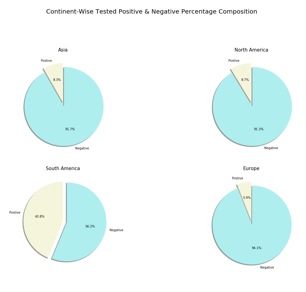

结论 (Conclusion)

Hurrah! We successfully completed creating our own COVID-19 report with Python. If you forgot to follow any above mentioned steps I have provided the full code for this analysis below. Apart from our analysis, there are much more you can do with Python and its powerful packages. So don’t stop exploring and create your own reports and dashboards.

欢呼！ 我们已经成功地使用Python创建了自己的COVID-19报告。 如果您忘记了执行上述任何步骤，则在下面提供了此分析的完整代码。 除了我们的分析之外，Python及其强大的软件包还可以做更多的事情。 因此，不要停止探索并创建自己的报告和仪表板。

You can find many useful resources on internet based on data science in python for example edX, Coursera, Udemy and so on but, never ever stop learning. Hope you find this article useful and knowledgeable. Happy Analyzing!

您可以在python中基于数据科学在Internet上找到许多有用的资源，例如edX，Coursera，Udemy等，但永远都不要停止学习。 希望您发现本文有用且知识渊博。 分析愉快！

FULL CODE:

完整代码：

import pandas as pd
import matplotlib.pyplot as plt
import plotly.express as px
import numpy as np
import plotly
import plotly.graph_objects as go
import datetime as dt
import requests
from plotly.subplots import make_subplots# Getting Dataurl_request = requests.get("https://services1.arcgis.com/0MSEUqKaxRlEPj5g/arcgis/rest/services/Coronavirus_2019_nCoV_Cases/FeatureServer/1/query?where=1%3D1&outFields=*&outSR=4326&f=json")
url_json = url_request.json()
df = pd.DataFrame(url_json['features'])
df['attributes'][0]# Data Wrangling# a. transforming datadata_list = df['attributes'].tolist()
data = pd.DataFrame(data_list)
data.set_index('OBJECTID')
data = data[['Province_State','Country_Region','Last_Update','Lat','Long_','Confirmed','Recovered','Deaths','Active']]
data.columns = ('State','Country','Last Update','Lat','Long','Confirmed','Recovered','Deaths','Active')
data['State'].fillna(value = '', inplace = True)
data# b. cleaning datadef convert_time(t):t = int(t)return dt.datetime.fromtimestamp(t)data = data.dropna(subset = ['Last Update'])
data['Last Update'] = data['Last Update']/1000
data['Last Update'] = data['Last Update'].apply(convert_time)
data# Exploratory Data Analysis & Visualization# Our analysis contains 'Ranking countries and provinces', 'Time Series' and 'Classification and Distribution'# 1. Ranking countries and provinces
# a. Top 10 confirmed countries (Bubble plot)top10_confirmed = pd.DataFrame(data.groupby('Country')['Confirmed'].sum().nlargest(10).sort_values(ascending = False))
fig1 = px.scatter(top10_confirmed, x = top10_confirmed.index, y = 'Confirmed', size = 'Confirmed', size_max = 120,color = top10_confirmed.index, title = 'Top 10 Confirmed Cases Countries')
fig1.show()# b. Top 10 deaths countries (h-Bar plot)top10_deaths = pd.DataFrame(data.groupby('Country')['Deaths'].sum().nlargest(10).sort_values(ascending = True))
fig2 = px.bar(top10_deaths, x = 'Deaths', y = top10_deaths.index, height = 600, color = 'Deaths', orientation = 'h',color_continuous_scale = ['deepskyblue','red'], title = 'Top 10 Death Cases Countries')
fig2.show()# c. Top 10 recovered countries (Bar plot)top10_recovered = pd.DataFrame(data.groupby('Country')['Recovered'].sum().nlargest(10).sort_values(ascending = False))
fig3 = px.bar(top10_recovered, x = top10_recovered.index, y = 'Recovered', height = 600, color = 'Recovered',title = 'Top 10 Recovered Cases Countries', color_continuous_scale = px.colors.sequential.Viridis)
fig3.show()# d. Top 10 active countriestop10_active = pd.DataFrame(data.groupby('Country')['Active'].sum().nlargest(10).sort_values(ascending = True))
fig4 = px.bar(top10_active, x = 'Active', y = top10_active.index, height = 600, color = 'Active', orientation = 'h',color_continuous_scale = ['paleturquoise','blue'], title = 'Top 10 Active Cases Countries')
fig4.show()# e. Most affected states/provinces in largely affected countries
# Here we are going to extract top 4 affected countries' states data and plot it!# Firstly, aggregating data with our dataset :
# USA
topstates_us = data['Country'] == 'US'
topstates_us = data[topstates_us].nlargest(5, 'Confirmed')
# Brazil
topstates_brazil = data['Country'] == 'Brazil'
topstates_brazil = data[topstates_brazil].nlargest(5, 'Confirmed')
# India
topstates_india = data['Country'] == 'India'
topstates_india = data[topstates_india].nlargest(5, 'Confirmed')
# Russia
topstates_russia = data['Country'] == 'Russia'
topstates_russia = data[topstates_russia].nlargest(5, 'Confirmed')# Let's plot!
# USA
fig5 = go.Figure(data = [go.Bar(name = 'Active Cases', x = topstates_us['Active'], y = topstates_us['State'], orientation = 'h'),go.Bar(name = 'Death Cases', x = topstates_us['Deaths'], y = topstates_us['State'], orientation = 'h')
])
fig5.update_layout(title = 'Most Affected States in USA', height = 600)
fig5.show()
# Brazil
fig6 = go.Figure(data = [go.Bar(name = 'Recovered Cases', x = topstates_brazil['State'], y = topstates_brazil['Recovered']),go.Bar(name = 'Active Cases', x = topstates_brazil['State'], y = topstates_brazil['Active']),go.Bar(name = 'Death Cases', x = topstates_brazil['State'], y = topstates_brazil['Deaths'])
])
fig6.update_layout(title = 'Most Affected States in Brazil', barmode = 'stack', height = 600)
fig6.show()
# India
fig7 = go.Figure(data = [go.Bar(name = 'Recovered Cases', x = topstates_india['State'], y = topstates_india['Recovered']),go.Bar(name = 'Active Cases', x = topstates_india['State'], y = topstates_india['Active']),go.Bar(name = 'Death Cases', x = topstates_india['State'], y = topstates_india['Deaths'])
])
fig7.update_layout(title = 'Most Affected States in India', barmode = 'stack', height = 600)
fig7.show()
# Russia
fig8 = go.Figure(data = [go.Bar(name = 'Recovered Cases', x = topstates_russia['State'], y = topstates_russia['Recovered']),go.Bar(name = 'Active Cases', x = topstates_russia['State'], y = topstates_russia['Active']),go.Bar(name = 'Death Cases', x = topstates_russia['State'], y = topstates_russia['Deaths'])
])
fig8.update_layout(title = 'Most Affected States in Russia', barmode = 'stack', height = 600)
fig8.show()# 2. Time series of top affected countries
# We need a new data for this plot
# https://covid19.who.int/ follow the link for this link for the next dataset(you can find the download option on the bottomright of the map chart)
time_series = pd.read_csv('who_data.csv', encoding = 'ISO-8859-1')
time_series['Date_reported'] = pd.to_datetime(time_series['Date_reported'])# a. Covid-19 cases worldwide
# Firsty Data
time_series_dates = time_series.groupby('Date_reported').sum()# Let's Plot
# Cumulative cases
fig11 = go.Figure()
fig11.add_trace(go.Scatter(x = time_series_dates.index, y = time_series_dates[' Cumulative_cases'], fill = 'tonexty',line_color = 'blue'))
fig11.update_layout(title = 'Cumulative Cases Worldwide')
fig11.show()
# Cumulative death cases
fig12 = go.Figure()
fig12.add_trace(go.Scatter(x = time_series_dates.index, y = time_series_dates[' Cumulative_deaths'], fill = 'tonexty',line_color = 'red'))
fig12.update_layout(title = 'Cumulative Deaths Worldwide')
fig12.show()
# Daily new cases
fig13 = go.Figure()
fig13.add_trace(go.Scatter(x = time_series_dates.index, y = time_series_dates[' New_cases'], fill = 'tonexty',line_color = 'gold'))
fig13.update_layout(title = 'Daily New Cases Worldwide')
fig13.show()
# Daily death cases
fig14 = go.Figure()
fig14.add_trace(go.Scatter(x = time_series_dates.index, y = time_series_dates[' New_deaths'], fill = 'tonexty',line_color = 'hotpink'))
fig14.update_layout(title = 'Daily Death Cases Worldwide')
fig14.show()# b. Most Affected Countries over the time
# Data
# USA
time_series_us = time_series[' Country'] == ('United States of America')
time_series_us = time_series[time_series_us]
# Brazil
time_series_brazil = time_series[' Country'] == ('Brazil')
time_series_brazil = time_series[time_series_brazil]
# India
time_series_india = time_series[' Country'] == ('India')
time_series_india = time_series[time_series_india]
# Russia
time_series_russia = time_series[' Country'] == ('Russia')
time_series_russia = time_series[time_series_russia]
# Peru
time_series_peru = time_series[' Country'] == ('Peru')
time_series_peru = time_series[time_series_peru]# Let's plot
# Cumulative cases
fig15 = go.Figure()
fig15.add_trace(go.Line(x = time_series_us['Date_reported'], y = time_series_us[' Cumulative_cases'], name = 'USA'))
fig15.add_trace(go.Line(x = time_series_brazil['Date_reported'], y = time_series_brazil[' Cumulative_cases'], name = 'Brazil'))
fig15.add_trace(go.Line(x = time_series_india['Date_reported'], y = time_series_india[' Cumulative_cases'], name = 'India'))
fig15.add_trace(go.Line(x = time_series_russia['Date_reported'], y = time_series_russia[' Cumulative_cases'], name = 'Russia'))
fig15.add_trace(go.Line(x = time_series_peru['Date_reported'], y = time_series_peru[' Cumulative_cases'], name = 'Peru'))
fig15.update_layout(title = 'Time Series of Most Affected countries"s Cumulative Cases')
fig15.show()
# Cumulative death cases
fig16 = go.Figure()
fig16.add_trace(go.Line(x = time_series_us['Date_reported'], y = time_series_us[' Cumulative_deaths'], name = 'USA'))
fig16.add_trace(go.Line(x = time_series_brazil['Date_reported'], y = time_series_brazil[' Cumulative_deaths'], name = 'Brazil'))
fig16.add_trace(go.Line(x = time_series_india['Date_reported'], y = time_series_india[' Cumulative_deaths'], name = 'India'))
fig16.add_trace(go.Line(x = time_series_russia['Date_reported'], y = time_series_russia[' Cumulative_deaths'], name = 'Russia'))
fig16.add_trace(go.Line(x = time_series_peru['Date_reported'], y = time_series_peru[' Cumulative_deaths'], name = 'Peru'))
fig16.update_layout(title = 'Time Series of Most Affected countries"s Cumulative Death Cases')
fig16.show()
# Daily new cases
fig17 = go.Figure()
fig17.add_trace(go.Line(x = time_series_us['Date_reported'], y = time_series_us[' New_cases'], name = 'USA'))
fig17.add_trace(go.Line(x = time_series_brazil['Date_reported'], y = time_series_brazil[' New_cases'], name = 'Brazil'))
fig17.add_trace(go.Line(x = time_series_india['Date_reported'], y = time_series_india[' New_cases'], name = 'India'))
fig17.add_trace(go.Line(x = time_series_russia['Date_reported'], y = time_series_russia[' New_cases'], name = 'Russia'))
fig17.add_trace(go.Line(x = time_series_peru['Date_reported'], y = time_series_peru[' New_cases'], name = 'Peru'))
fig17.update_layout(title = 'Time Series of Most Affected countries"s Daily New Cases')
fig17.show()
# Daily death cases
fig18 = go.Figure()
fig18.add_trace(go.Line(x = time_series_us['Date_reported'], y = time_series_us[' New_deaths'], name = 'USA'))
fig18.add_trace(go.Line(x = time_series_brazil['Date_reported'], y = time_series_brazil[' New_deaths'], name = 'Brazil'))
fig18.add_trace(go.Line(x = time_series_india['Date_reported'], y = time_series_india[' New_deaths'], name = 'India'))
fig18.add_trace(go.Line(x = time_series_russia['Date_reported'], y = time_series_russia[' New_deaths'], name = 'Russia'))
fig18.add_trace(go.Line(x = time_series_peru['Date_reported'], y = time_series_peru[' New_deaths'], name = 'Peru'))
fig18.update_layout(title = 'Time Series of Most Affected countries"s Daily Death Cases')
fig18.show()# 3. Case Classification and Distribution# For this we need a new dataset
# https://www.kaggle.com/imdevskp/corona-virus-report follow this link for the next dataset# a. WHO Region-Wise Distribution
# For this plot we are going to use country_wise_latest dataset which will come along with the downloaded kaggle dataset
# Firstly Data
who = pd.read_csv('country_wise_latest.csv')
who_region = pd.DataFrame(who.groupby('WHO Region')['Confirmed'].sum())
labels = who_region.index
values = who_region['Confirmed']
# Let's Plot!
fig9 = go.Figure(data=[go.Pie(labels = labels, values = values, pull=[0, 0, 0, 0, 0.2, 0])])
fig9.update_layout(title = 'WHO Region-Wise Case Distribution', width = 700, height = 400, margin = dict(t = 0, l = 0, r = 0, b = 0))
fig9.show()# b. Most Affected countries case distribution
# For this plot we are going to use the same country_wise_latest dataset# Firstly Data
case_dist = who
# US
dist_us = case_dist['Country/Region'] == 'US'
dist_us = case_dist[dist_us][['Country/Region','Deaths','Recovered','Active']].set_index('Country/Region')
# Brazil
dist_brazil = case_dist['Country/Region'] == 'Brazil'
dist_brazil = case_dist[dist_brazil][['Country/Region','Deaths','Recovered','Active']].set_index('Country/Region')
# India
dist_india = case_dist['Country/Region'] == 'India'
dist_india = case_dist[dist_india][['Country/Region','Deaths','Recovered','Active']].set_index('Country/Region')
# Russia
dist_russia = case_dist['Country/Region'] == 'Russia'
dist_russia = case_dist[dist_russia][['Country/Region','Deaths','Recovered','Active']].set_index('Country/Region')# Let's Plot!
# This plot is produced with matplotlib
fig = plt.figure(figsize = (22,14))
colors_series = ['deepskyblue','gold','springgreen','coral']
explode = (0,0,0.1)plt.subplot(221)
plt.pie(dist_us, labels = dist_us.columns, colors = colors_series, explode = explode,startangle = 90,autopct = '%.1f%%', shadow = True)
plt.title('USA', fontsize = 16)plt.subplot(222)
plt.pie(dist_brazil, labels = dist_brazil.columns, colors = colors_series, explode = explode,startangle = 90,autopct = '%.1f%%',shadow = True)
plt.title('Brazil', fontsize = 16)plt.subplot(223)
plt.pie(dist_india, labels = dist_india.columns, colors = colors_series, explode = explode, startangle = 90, autopct = '%.1f%%',shadow = True)
plt.title('India', fontsize = 16)plt.subplot(224)
plt.pie(dist_russia, labels = dist_russia.columns, colors = colors_series, explode = explode, startangle = 90,autopct = '%.1f%%', shadow = True)
plt.title('Russia', fontsize = 16)plt.suptitle('Case Classification of Most Affected Countries', fontsize = 20)# c. Most affected continents' negative case vs positive case percentage composition
# For this we need a new dataset
# https://ourworldindata.org/coronavirus-source-data Follow this link for our next dataset# Firstly Data
negative_positive = pd.read_csv('owid-covid-data.csv')
negative_positive = negative_positive.groupby('continent')[['total_cases','total_tests']].sum()
explode = (0,0.1)
labels = ['Postive','Negative']
colors = ['beige','paleturquoise']#Let's Plot!
fig = plt.figure(figsize = (20,20))
plt.subplot(321)
plt.pie(negative_positive[negative_positive.index == 'Asia'],labels = labels, explode = explode, autopct = '%.1f%%', startangle = 90, colors = colors, shadow = True)
plt.title('Asia', fontsize = 15)plt.subplot(322)
plt.pie(negative_positive[negative_positive.index == 'North America'],labels = labels, explode = explode, autopct = '%.1f%%', startangle = 90, colors = colors, shadow = True)
plt.title('North America', fontsize = 15)plt.subplot(323)
plt.pie(negative_positive[negative_positive.index == 'South America'],labels = labels, explode = explode, autopct = '%.1f%%', startangle = 90, colors = colors, shadow = True)
plt.title('South America', fontsize = 15)plt.subplot(324)
plt.pie(negative_positive[negative_positive.index == 'Europe'],labels = labels, explode = explode, autopct = '%.1f%%', startangle = 90, colors = colors, shadow = True)
plt.title('Europe', fontsize = 15)plt.suptitle('Continent-Wise Tested Positive & Negative Percentage Composition', fontsize = 20)