The caption in the online magazine “WIRED” caught my eye one night a few months ago. When I focused my eyes on it, it read: “Can everything be explained to everyone in terms they can understand? In 5 Levels, an expert scientist explains a high-level subject in five different layers of complexity - first to a child, then a teenager, then an undergrad majoring in the same subject, a grad student, and finally, a colleague”.

几个月前一个晚上，在线杂志“ WIRED”的标题引起了我的注意。 当我将目光聚焦在它上面时，它写着：“ 可以用每个人都能理解的术语向所有人解释一切吗？ 在5个级别中，一位专家科学家通过五个不同层次的复杂性解释了一个高级主题 - 首先是给孩子，然后是少年，然后是主修同一主题的本科生，然后是研究生，最后是同事 ”。

Curious, I clicked on the link and started learning about exciting new concepts I could finally grasp with my own level of understanding. Music, Biology, Physics, Medicine - all seemed clear that night. Needless to say, I couldn’t stop watching the series and went to bed very very late.

很好奇，我单击了链接，开始学习一些令人兴奋的新概念，这些新概念最终将以我自己的理解水平掌握。 音乐，生物学，物理学，医学-那天晚上似乎都很清楚。 不用说，我无法停止观看该系列节目，而且非常晚才上床睡觉。

I actually started writing this article while working on a more technical piece. From a few paragraphs in the text, it grew in size until I felt my original article could no longer hold its weight. Could I explain the key concepts to peers and to co-workers, as well as to children and people without mathematical orientation? How far along will readers follow the explanations?

我实际上是在撰写更多技术文章时开始写这篇文章的。 从文本中的几段开始，它的大小不断增加，直到我觉得我的原始文章不再能承受它的重量。 我能否向同龄人和同事以及没有数学知识的孩子和人们解释关键概念？ 读者将遵循这些解释多远？

Let’s find out :)

让我们找出来:)

1) Child

1)儿童

Sometimes, when we learn new things, we are told lots of facts and might be shown a drawing or a table with numbers. Seeing a lot of numbers and tables can be confusing, so it would be really helpful if we could reach the same conclusions, just using less of these facts, tables, and numbers.

有时，当我们学习新事物时，会被告知很多事实，并可能会看到带有数字的图形或表格。 看到大量的数字和表格可能会造成混淆，因此，如果我们能够使用较少的事实，表格和数字得出相同的结论，那将非常有帮助。

Principal Component Analysis (or PCA for short) is what we call an algorithm: a set of instructions to follow. If we represent all our facts and tables using numbers, following these instructions will allow us to represent them using fewer numbers.

主成分分析(或简称PCA)是我们所谓的算法：一组遵循的指令。 如果我们使用数字表示所有事实和表格，则按照以下说明进行操作可以使我们使用较少的数字表示它们。

If we convert these numbers back into facts, we can still draw the same conclusions. But because we drew them using fewer facts than before, performing PCA just helped us be less confused.

如果将这些数字转换为事实，我们仍然可以得出相同的结论。 但是，因为我们使用的事实比以前更少了，所以执行PCA可以减少我们的困惑。

2) High-school aged teenager

2)高中生

Our math studies focus on a few key areas that give us a basis for mathematical understanding and orientation. High school math often means learning Calculus, which deals with subjects like function analysis and analytic geometry. Let’s use them to better explain Principal Component Analysis.

我们的数学研究集中在几个关键领域，这些领域为我们提供了数学理解和定向的基础。 高中数学通常意味着学习微积分，它涉及功能分析和解析几何等主题。 让我们用它们更好地解释主成分分析。

Functions are special objects in mathematics that give us an output value when we feed it an input value. This makes them very useful in learning certain relationships in data. A key technique taught in high school is how to draw the graph of a function by performing a short analysis of its properties. We use something from Calculus called the Derivative: A derivative is just an approximation of the slope of a function at a given point. We choose a few key points inside the area of our graph to find the values our function will take at these points and calculate the derivative of the function at these points to get hints about the slope of the function. Then we use the points and the slopes we just got to draw an approximation of the function’s shape.

函数是数学中的特殊对象，当我们将输入值提供给输入值时，函数会为我们提供输出值。 这使得它们在学习数据中的某些关系时非常有用。 高中教授的一项关键技术是如何通过对功能的简短分析来绘制功能图。 我们使用微积分中的一种叫做导数的东西：导数只是一个函数在给定点的斜率的近似值。 我们在图形区域内选择一些关键点，以查找函数在这些点处采用的值，并在这些点处计算函数的导数，以获取有关函数斜率的提示。 然后，我们使用得到的点和斜率来绘制函数形状的近似值。

In the real world, sometimes we have lots of functions and even strange things like functions that output multiple values at the same time or functions that require multiple inputs to give us values. And if you are the kind of person that finds high school functions dreadful, imagine how dreadful these multi-number functions can be — even for skilled adults! Principal component analysis is a technique that takes the output for all these functions and gives us close approximations using much less of these numbers. Fewer numbers often mean memorizing less data, smaller and cheaper ways to store them, and less of that “being confused” feeling we get when we see so many numbers we don’t even know where to start.

在现实世界中，有时我们有很多功能，甚至有些奇怪的事情，例如同时输出多个值的功能或需要多个输入才能为我们提供值的功能。 而且，如果您是那种对高中职能感到恐惧的人，请想象一下，即使对于熟练的成年人来说，这些多重数字功能可能有多么可怕！ 主成分分析是一种获取所有这些函数的输出并使用更少的这些数字为我们提供近似值的技术。 数字越少，通常意味着要记住的数据越少，存储数据的方式越小越便宜，并且当我们看到如此多的数字甚至不知道从哪里开始时，就会感到越来越“困惑”。

3) First-year University student

3)大学一年级学生

During your studies, you’ve learned all about linear algebra, statistics, and probability. You’ve dealt with a few of these “real world” functions that input and output multiple values and learned that they work with these things called vectors and matrices. You’ve also learned all about random variables, sample values, means, variances, distributions, covariances, correlation, and all the rest of the statistics techno-babble.

在学习期间，您已经了解了线性代数，统计量和概率的全部知识。 您已经处理了其中一些输入和输出多个值的“真实世界”函数，并了解到它们可用于矢量和矩阵。 您还了解了有关随机变量，样本值，均值，方差，分布，协方差，相关性以及所有其他统计技术tech语的知识。

Principal Component Analysis relies on a technique called “Singular value decomposition” (SVD for short). For now let’s treat it as what’s called a “black box” in computer science: an unknown function that gives us some desired output once we feed it with the required input. If we collect lots of data (from observations, experimentation, monitoring etc…) and store it in matrix form, we can input this matrix to our SVD function and get a matrix of smaller dimensions that allows us to represent our data with fewer values.

主成分分析依赖于称为“奇异值分解”(简称SVD)的技术。 现在，让我们将其视为计算机科学中的“黑匣子”：一个未知函数，一旦我们将其输入所需的输入，便会提供一些所需的输出。 如果我们收集大量数据(来自观察，实验，监视等)并将其以矩阵形式存储，则可以将此矩阵输入到SVD函数中，并获得较小尺寸的矩阵，该矩阵可以用更少的值表示数据。

While for now, it might make sense to keep the SVD as a black box, it could be interesting to investigate the input and output matrices further. And it turns out the SVD gives us extra-meaningful outputs for a special kind of matrix called a “covariance matrix”. Being an undergrad student, you’ve already dealt with covariance matrices, but you might be thinking: “What does my data have to do with them?”

虽然目前将SVD保留为黑匣子可能是有意义的，但进一步研究输入和输出矩阵可能会很有趣。 事实证明，SVD为我们提供了一种称为“协方差矩阵”的特殊矩阵，对我们来说意义非凡。 作为本科生，您已经处理过协方差矩阵，但是您可能会想：“我的数据与它们有什么关系？”

Our data actually has quite a lot to do with covariance matrices. If we sort our data into distinct categories, we can group related values in a vector representing that category. Each one of these vectors can also be seen as a random variable, containing n samples (which makes n the length of the vector). If we concatenate these vectors together, we can form a matrix X of m random variables, or a random vector with m scalars, holding n measurements of that vector.

实际上，我们的数据与协方差矩阵有很大关系。 如果我们将数据分类为不同的类别，则可以将相关值分组在代表该类别的向量中。 这些向量中的每一个也可以看作是一个随机变量，包含n个样本(使向量的长度为n)。 如果将这些向量连接在一起，我们可以形成m个随机变量的矩阵X，或者形成一个m个标量的随机向量，并对该向量进行n次测量。

The matrix of concatenated vectors, representing our data, can then be used to calculate the covariance matrix for our random vector. This matrix is then provided as an input for our SVD, which provides us with a unitary matrix as an output.

表示我们数据的级联向量矩阵可用于计算随机向量的协方差矩阵。 然后将此矩阵作为我们SVD的输入，后者为我们提供了一个matrix矩阵作为输出。

Without diving in too deep into unitary matrices, the output matrix has a neat property: we can pick the first k column vectors from the matrix to generate a new matrix U, and multiply our original matrix X with the matrix U to obtain a lower-dimensional matrix. It turns out this matrix is the “best” representation of the data stored in X when mapped to a lower dimension.

在不深入探讨unit矩阵的情况下，输出矩阵具有简洁的属性：我们可以从矩阵中选取前k个列向量来生成新矩阵U，然后将原始矩阵X与矩阵U相乘以获得较低的-尺寸矩阵。 事实证明，当映射到较低维度时，此矩阵是存储在X中的数据的“最佳”表示。

4) Bachelor of Science

4)理学学士

Graduating with an academic degree, you now have the mathematical background needed to properly explain Principal component analysis. But just writing down the math won’t be helpful if we don’t understand the intuition behind it or the problem we are trying to solve.

通过学习，您现在拥有正确解释主成分分析所需的数学背景。 但是，如果我们不了解其背后的直觉或我们试图解决的问题，则仅写下数学将无济于事。

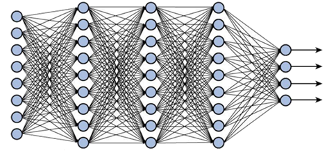
The problem PCA tries to solve is what we nickname the “curse of dimensionality”: When we try to train machine learning algorithms, the rule of thumb is that the more data we collect, the better our predictions become. But with every new data feature (implying we now have an additional random vector) the dimension of the vector space spanned by the feature vectors increases by one. The larger our vector space, the longer it takes to train our learning algorithms, and the higher the chance some of the data might be redundant.

PCA试图解决的问题是我们昵称的“维数诅咒”：当我们尝试训练机器学习算法时，经验法则是，我们收集的数据越多，我们的预测就越好。 但是，对于每个新的数据特征(这意味着我们现在有了一个附加的随机向量)，特征向量跨越的向量空间的维数将增加一。 向量空间越大，训练我们的学习算法所需的时间就越长，并且某些数据可能是多余的机会也就越大。

To solve this, researchers and mathematicians have constantly been trying to find techniques that perform “dimensionality reduction”: embedding our vector space in another space with a lower dimension. The inherent problem in dimensionality reductions is that for every decrease in the dimension of the vector space, we essentially discard one of the random vectors spanning the original vector space. That is because the basis for the new space has one vector less, making one of our random vectors a linear combination of the others, and therefore redundant in training our algorithm.

为了解决这个问题，研究人员和数学家一直在努力寻找执行“降维”的技术：将向量空间嵌入到另一个具有较小维度的空间中。 降维的固有问题是，向量空间尺寸的每减小一次，我们实际上就丢弃了跨越原始向量空间的随机向量之一。 那是因为新空间的基础少了一个向量，使我们的随机向量之一成为其他向量的线性组合，因此在训练我们的算法时是多余的。

Of course, we do have naïve techniques for dimensionality reduction (like just discarding random vectors and checking which lost vector has the smallest effect on the accuracy of the algorithm). But the question asked is “How can I lose the least information when performing dimensionality reduction?” And it turns out the answer is “By using PCA”.

当然，我们确实有用于降维的幼稚技术(就像只是丢弃随机向量并检查哪个丢失的向量对算法的精度影响最小)。 但是问的问题是“执行降维时如何丢失最少的信息？” 事实证明，答案是“通过使用PCA”。

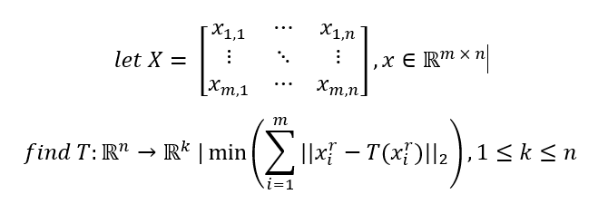
Formulating this mathematically, if we represent our data in matrix form as we did before, with n random variables having m measurements each, we represent each sample as the row xi. We are therefore searching for a linear map T: ℝn → ℝk that minimizes the Euclidian distances between xi and T(xi)

用数学公式表示，如果我们像以前一样以矩阵形式表示数据，则n个随机变量各具有m个测量值，我们将每个样本表示为xi行。 因此，我们正在寻找一个线性映射T： ℝn → ℝk ，它使xi与T(xi)之间的欧几里得距离最小

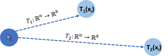
The intuition behind this formulation is that if we represent our image vectors as n-dimensional vectors in the original vector space, the less they have moved from their original positions implies the smaller the loss of information. Why does distance imply loss of information? Because the closer a representation of a vector is to its original location, the more accurate the representation.

这种表述的直觉是，如果我们将图像矢量表示为原始矢量空间中的n维矢量，则它们从其原始位置移出的次数越少，则意味着信息损失越小。 为什么距离意味着信息丢失？ 因为矢量的表示越接近其原始位置，表示就越准确。

How do we find that linear map? It turns out that the map is provided by the Singular value decomposition! Recall that if we invoke SVD we obtain a unitary matrix U that satisfies

我们如何找到线性图？ 事实证明，映射是由奇异值分解提供的！ 回想一下，如果调用SVD，我们将获得一个满足的matrix矩阵U

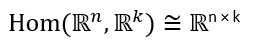
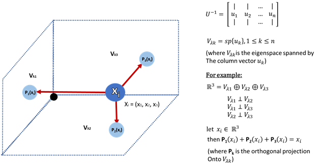
Due to the isomorphism between the linear map space and the matrix space, we can see the matrix U as representing a linear map from ℝn to ℝn:

由于线性图空间和矩阵空间之间的同构，我们可以看到矩阵U表示从ℝn到ℝn的线性图：

How exactly does SVD provide us with the function U? SVD is essentially a generalization of an important theorem in linear algebra called the Spectral theorem. While the spectral theorem can only be applied to normal matrices (satisfying MM* = M*M, where M* is the complex conjugate of M), SVD generalizes that result to any arbitrary matrix M, by performing a matrix decomposition into three matrices: SVD(M) = U*Σ*V.

SVD如何为我们提供函数U？ SVD本质上是线性代数中一个重要定理的泛化，称为谱定理。 虽然频谱定理仅适用于正常矩阵(满足MM * = M * M，其中M *是M的复共轭)，但SVD通过将矩阵分解为三个矩阵将结果归纳为任意矩阵M： SVD(M)= U *Σ* V。

According to the Spectral theorem, U is a unitary matrix whose row vectors are an orthonormal basis for Rn, with each row vector spanning an eigenspace orthogonal to the other eigenspaces. If we denote that basis as B = {u1, u2 … un}, And because U diagonalizes the matrix M, it can also be viewed as a transformation matrix between the standard basis and the basis B.

根据谱定理，U是一个ary矩阵，其行向量是Rn的正交基础，每个行向量都跨越与其他本征空间正交的本征空间。 如果我们将该基准表示为B = {u1，u2…un}，并且由于U将矩阵M对角化，则它也可以看作是标准基准和基准B之间的转换矩阵。

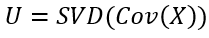
Of course, any subset Bk = {u1, u2 … uk} is an orthonormal basis for ℝ(k). This means that performing the multiplication M * U-1 (similar to multiplying U * M) is isomorphic to a linear map T: ℝn → ℝk. The theorems behind SVD generalizes this result to any given matrix. And while these matrices aren’t necessarily diagonalizable (or even square), the results regarding the unitary matrices still hold true for U and V. All we have left is to perform the multiplication X’ = Cov(X) * U, performing the dimensionality reduction we were searching for. We can now use the reduced matrix X’ for any purpose we’d have used the original matrix X for.

当然，任何子集Bk = {u1，u2…uk}是ℝ (k)的正交基础。 这意味着，在执行乘法M * U-1(类似于乘以U * M)是同构的线性地图T：ℝÑ→ℝķ。 SVD背后的定理将这个结果推广到任何给定的矩阵。 尽管这些矩阵不一定是对角线化的(甚至平方)，但有关U和V的the矩阵的结果仍然成立。剩下的就是执行乘法X'= Cov(X)* U，然后执行我们正在寻找的降维。 现在，我们可以将缩减后的矩阵X'用于原始矩阵X所用于的任何目的。

5) Expert data scientist

5)专家数据科学家

As an expert data scientist with a hefty amount of experience in research and development of learning algorithms, you probably already know of PCA and don’t need abridged descriptions of its internal workings and of applying it in practice. I do find however that many times, even when we have been applying an algorithm for a while, we don’t always know the math that makes it work.

作为在学习算法的研究和开发方面拥有大量经验的专家数据科学家，您可能已经了解PCA，不需要对其内部工作以及在实践中应用它的简要说明。 但是，我确实发现很多次，即使我们已经应用了一段时间的算法，我们也不总是知道使它起作用的数学方法。

If you’ve followed along with the previous explanations, we still have two questions left: Why does the matrix U represent the linear map T which minimizes the loss of information? And how does SVD provide us with such a matrix U?

如果您按照前面的说明进行操作，那么我们还有两个问题：为什么矩阵U代表线性映射T，从而将信息损失降至最低？ SVD如何为我们提供这样的矩阵U？

The answer to the first question lies in an important result in linear algebra called the Principal Axis theorem. It states that every ellipsoid (or hyper-ellipsoid equivalent) shape in analytic geometry can be represented as a quadratic form Q: ℝn x ℝn → ℝ of the shape Q(x)=x’Ax, (here x’ denotes the transpose of x) such that A is diagonalizable and has a spectral decomposition into mutually orthogonal eigenspaces. The eigenvectors obtained form an orthonormal basis of ℝn, and have the property of matching the axes of the hyper-ellipsoid. That’s neat!

第一个问题的答案在于线性代数的一个重要结果，称为主轴定理。 它指出解析几何中的每个椭球(或超椭球等效)形状都可以表示为二次形式Q： ℝn xℝn → ℝ形状Q(x)= x'Ax，(此处x'表示转置的x)，使得A可对角化并在光谱上分解为相互正交的本征空间。 形式ℝn的正交基所获得的特征向量，并具有超椭圆体的轴相匹配的属性。 那很整齐！

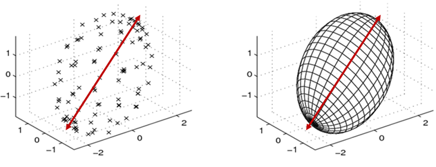
The Principal Axis theorem shows a fundamental connection between linear algebra and analytic geometry. When plotting our matrix X and visualizing the individual values, we can plot a (roughly) hyper-ellipsoid shape containing our data points. We can then plot a regression line for each dimension of our data, trying to minimize the distance to the orthogonal projection of the data points onto the regression line. Due to the properties of hyper-ellipsoids, these lines are exactly their axes. Therefore, the regression lines correspond to the spanning eigenvectors obtained from the spectral decomposition of the quadratic form Q.

主轴定理显示了线性代数与解析几何之间的基本联系。 在绘制矩阵X并可视化各个值时，我们可以绘制一个包含数据点的(大致)超椭圆形。 然后，我们可以为数据的每个维度绘制一条回归线，以尽量减少到数据点在回归线上的正交投影的距离。 由于超椭圆体的特性，这些线正好是它们的轴。 因此，回归线对应于从二次形式Q的光谱分解中获得的跨越特征向量。

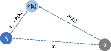
Reviewing a diagram similar to the one used when formulating the problem, notice the tradeoff between the length of an orthogonal projection to the length of its orthogonal complement: The smaller the orthogonal complement, the larger the orthogonal projection. Even though X is written in matrix form, we must not forget it is a random vector, and as such its components exhibit variance between their measurements. Since P(x) is a projection, it inevitably loses some information about x, which accumulates to a loss of variance.

查看与解决问题时使用的示意图类似的图，请注意正交投影的长度与其正交补角的长度之间的折衷：正交补角越小，正交投影就越大。 即使X以矩阵形式编写，我们也不能忘记它是一个随机向量，因此它的分量在它们的测量之间表现出方差。 由于P(x)是一个投影，它不可避免地会丢失一些有关x的信息，从而累积了方差损失。

In order to minimize the variance lost (i.e. retain the maximum possible variance) across the orthogonal projections, we must minimize the length of the orthogonal complements. Since the regression lines coinciding with our data’s principal axes minimizes the orthogonal complements of the vectors representing our measurements, they also maximize the amount of variance kept from the original vectors. This is exactly why SVD “minimizes the loss of information”: because it maximizes the variance kept.

为了最小化正交投影上损失的方差(即，保持最大可能的方差)，我们必须最小化正交互补序列的长度。 由于与我们数据主轴一致的回归线使代表我们测量值的矢量的正交补数最小，因此它们也使与原始矢量保持的方差量最大化。 这就是SVD“最大程度地减少信息丢失”的原因：因为它最大程度地保持了差异。

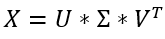
Now that we’ve discussed the theory behind SVD, how does it do its magic? SVD takes a matrix X as it’s input, and decomposes it into three matrices: U, Σ, and V, that satisfy X = U*Σ*V. Since SVD is a decomposition rather than a theorem, let’s perform it step by step on the given matrix X.

既然我们已经讨论了SVD背后的理论，那么它如何发挥作用呢？ SVD将矩阵X作为输入，并将其分解为三个矩阵：U，Σ和V，它们满足X = U *Σ* V。 由于SVD是分解而不是定理，因此让我们在给定的矩阵X上逐步执行它。

First, we’re going to introduce a new term: a Singular vector of a matrix is any vector v that satisfies the equation

首先，我们将引入一个新术语：矩阵的奇异向量是满足等式的任何向量v

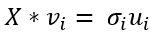
Since X ∈ ℝ(m x n), we have no guarantees as to its dimensions or its contents. X might not have eigenvalues (since eigenvalues are only defined for square matrices), but it always has at least ρ different singular vectors (with ρ(X) being the rank of X), each with a matching singular value.

由于X∈ℝ (mxn)，因此我们无法保证其尺寸或内容。 X可能没有特征值(因为特征值仅针对平方矩阵定义)，但它始终至少具有ρ个不同的奇异矢量(其中ρ(X)是X的秩)，每个奇异矢量都具有匹配的奇异值。

We can then use X to construct a symmetric matrix

然后我们可以使用X来构造对称矩阵

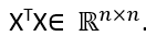
Since every transposed matrix is also an adjoint matrix, the singular values of XT are the complex conjugates of the singular values of X. This makes each eigenvalue of XT*X the square of the matching singular value of X:

由于每个转置矩阵也是一个伴随矩阵，因此XT的奇异值是X的奇异值的复共轭。这使XT * X的每个特征值成为X的匹配奇异值的平方：

Because XT*X is symmetric, it is also normal. Therefore, XT*X is orthogonally diagonalizable: There exists a diagonal matrix Σ2 which can be written as a product of three matrices:

由于XT * X是对称的，因此也是正常的。 因此，XT * X可正交对角化：存在一个对角矩阵Σ2，可以将其写为三个矩阵的乘积：

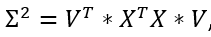
where V is an orthonormal matrix made of eigenvectors of XTX. We will mark these vectors as

其中V是由XTX特征向量组成的正交矩阵。 我们将这些向量标记为

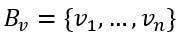
We now construct a new group of vectors

现在，我们构建一组新的向量

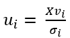
where we define each member as

我们将每个成员定义为

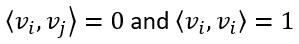
Notice that because Bv is an orthonormal group, for every 1≤i≤j≤n

注意，由于Bv是一个正交群，所以每1≤i≤j≤n

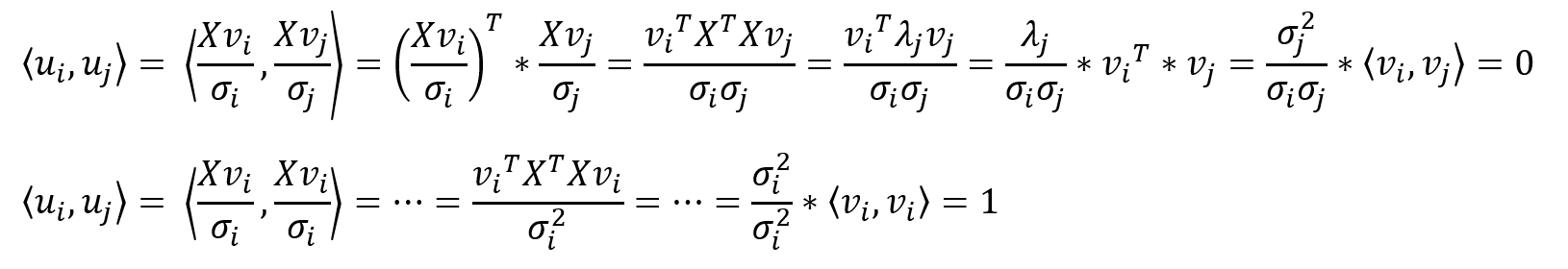
Therefore, we can prove that:

因此，我们可以证明：

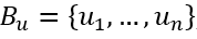
In addition, ui is also an eigenvector of X*XT: This is because

另外，ui也是X * XT的特征向量：这是因为

We can now complete the proof by expressing the relationship between Bu and Bv in matrix form:

现在，我们可以通过以矩阵形式表示Bu和Bv之间的关系来完成证明：

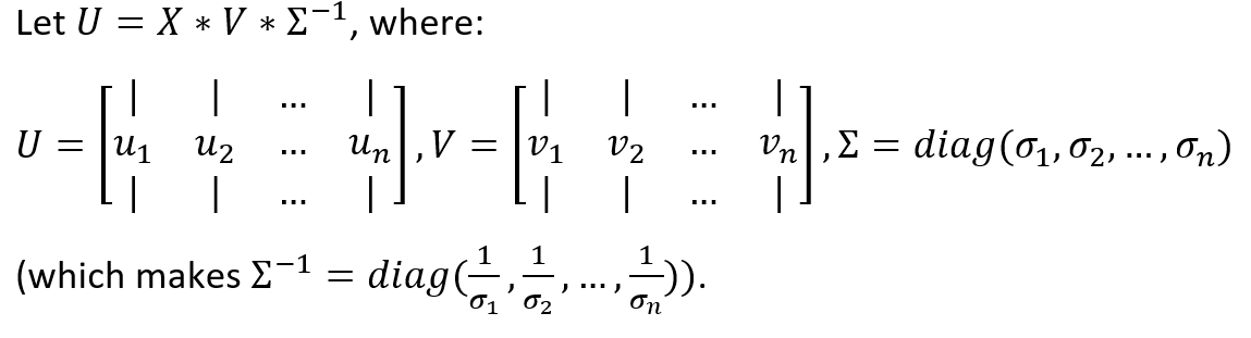
Then by standard matrix multiplication: U*Σ=X*V, and it immediately follows that

然后通过标准矩阵乘法：U *Σ= X * V，它紧随其后

The result we just achieved is impressive, but remember we constructed Bu as a group of n vectors using the vectors of Bv, meaning U∈R(m×n) while Σ∈ R(n×n). While this is a valid multiplication, U is not a square matrix and therefore cannot be a unitary matrix. To solve this, we “pad” the matrix Σ with zeros to achieve an m×n shape and extend U to an m×m shape using the Gram-Schmidt process.

我们刚刚获得的结果令人印象深刻，但请记住，我们使用Bv的向量将Bu构造为n个向量的组，这意味着U∈R(m×n)而Σ∈R(n×n)。 虽然这是一个有效的乘法，但U不是方矩阵，因此不能是a矩阵。 为了解决这个问题，我们用零“填充”矩阵Σ以得到m×n形状，并使用Gram-Schmidt过程将U扩展为m×m形状。

Now that we’ve finished the math part (phew…), we can start drawing some neat connections. First, while SVD can technically decompose any matrix, and we could just feed in the raw data matrix X, the Principal Axis theorem only works for diagonalizable matrices.

现在我们已经完成了数学部分((…)，我们可以开始绘制一些整洁的连接了。 首先，虽然SVD可以从技术上分解任何矩阵，并且我们可以只输入原始数据矩阵X，但主轴定理仅适用于可对角矩阵。

Second, the Principal axis theorem maximizes the retained variance in our matrix by performing an orthogonal projection onto the matrix’s eigenvectors. But who said our matrix captured a good amount of variance in the first place?

其次，主轴定理通过对矩阵的特征向量进行正交投影，使矩阵中的保留方差最大化。 但是谁说我们的矩阵首先捕获了大量的方差呢？

To answer these questions, and bring this article to an end, we will first restate that capturing variance between random variables is done by using a covariance matrix. And because the covariance matrix is symmetric and positive semi-definite, it is orthogonally diagonalizable AND has a spectral decomposition. We can then rewrite the formula for the covariance matrix using this neat equation, obtained by applying SVD to the matrices multiplied to form the covariance matrix:

为了回答这些问题并结束本文，我们将首先重申使用协方差矩阵来捕获随机变量之间的方差。 并且因为协方差矩阵是对称且正半定的，所以它可以正交对角化并且具有频谱分解。 然后，我们可以使用这个整齐的方程式重写协方差矩阵的公式，该方程是通过将SVD应用于乘以形成协方差矩阵的矩阵而获得的：

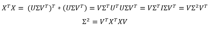
This is exactly why we said that SVD gives us extra-meaningful outputs when being applied to the covariance matrix of X:

这就是为什么我们说SVD应用于X的协方差矩阵时会给我们额外的意义：

a) Not only is the Singular Value decomposition of Cov(X) is identical to its Spectral decomposition, it diagonalizes it!

a)Cov(X)的奇异值分解不仅与其频谱分解相同，而且对角化！

b) The diagonalizing matrix V is an orthonormal matrix made of unitary eigenvectors of Cov(X), which is used to perform the Principal component analysis of X!

b)对角化矩阵V是由Cov(X)的单一特征向量组成的正交矩阵，用于执行X！的主成分分析！

c) Using Cov(X) captures the maximum amount of variance in our data, and by projecting it onto the basis eigenvectors associated with the k-largest eigenvalues of Cov(X) we lose the smallest possible amount of variance for reducing our data by (n-k) dimensions

c)使用Cov(X)捕获数据中的最大方差量，并将其投影到与Cov(X)的k个最大特征值相关的基础特征向量上，我们损失了最小的方差量来减少我们的数据(nk)尺寸

d) The Principal Axis theorem ensures that we minimize the projection error from ℝn→ℝk when performing PCA using Cov(X) and V.

d)主轴定理确保当使用Cov(X)和V执行PCA时，使从ℝn → ℝk引起的投影误差最小。