python——聚类
目录
- Cluster Analysis聚类分析
- Introduction to Unsupervised Learning无监督学习简介
- Clustering
- Distance or Similarity Function距离或相似度函数
- Clustering as an Optimization Problem聚类是一个优化问题
- Types of Clustering聚类的类型
- Partitioning Method
- KMeans
- KMeans Algorithm
- KMeans
- KMeans算法
- Limitations of KMeans.KMeans的局限性
- Meanshift
- Hierarchial Clustering层次集群
- Agglomerative method凝聚法
- Density Based Clustering - DBSCAN
- Measuring Performance of Clusters衡量聚类的性能
- completeness_score
- homogeneity_score
- silhoutte_score
- Example : Selecting the number of clusters with silhouette analysis on KMeans clustering
- calinski_harabaz_score
Cluster Analysis聚类分析
- Introduction to Unsupervised Learning
- Clustering
- Similarity or Distance Calculation
- Clustering as an Optimization Function
- Types of Clustering Methods
- Partitioning Clustering - KMeans & Meanshift
- Hierarchial Clustering - Agglomerative
- Density Based Clustering - DBSCAN
- Measuring Performance of Clusters
1.无监督学习简介
2.聚类
3.相似度或距离计算
4.聚类作为优化函数
5.聚类方法的类型
6.分区聚类-KMeans和Meanshift
7.层次聚类-聚集
8.基于密度的群集-DBSCAN
9.衡量集群的绩效
10.比较所有聚类方法
Introduction to Unsupervised Learning无监督学习简介
- Unsupervised Learning is a type of Machine learning to draw inferences from unlabelled datasets.
- Model tries to find relationship between data.
- Most common unsupervised learning method is clustering which is used for exploratory data analysis to find hidden patterns or grouping in data
- 无监督学习是一种机器学习,可以从未标记的数据集中得出推论。
- 模型试图查找数据之间的关系。
- 最常见的无监督学习方法是聚类,用于探索性数据分析以发现隐藏模式或数据分组
Clustering
A learning technique to group a set of objects in such a way that objects of same group are more similar to each other than from objects of other group.
Applications of clustering are as follows
- Automatically organizing the data
- Labeling data
- Understanding hidden structure of data
- News Cloustering for grouping similar news together
- Customer Segmentation
- Suggest social groups
一种将一组对象进行分组的学习技术,使得同一组的对象比来自其他组的对象彼此更相似。
集群的应用如下:
- 自动整理数据
- 标签数据
- 了解数据的隐藏结构
- 新闻汇总,将相似的新闻分组在一起
- 客户细分
- 建议社交团体
import numpy as np
import pandas as pd
import matplotlib.pyplot as plt
%matplotlib inline
from sklearn.datasets import make_blobs#make_blobs 产生多类数据集,对每个类的中心和标准差有很好的控制
- Generating natural cluster
- 生成自然簇
X,y = make_blobs(n_features=2, n_samples=1000, centers=3, cluster_std=1, random_state=3)
plt.scatter(X[:,0], X[:,1], s=5, alpha=.5)
![]()
Distance or Similarity Function距离或相似度函数
- Data belonging to same cluster are similar & data belonging to different cluster are different.
- We need mechanisms to measure similarity & differences between data.
- This can be achieved using any of the below techniques.
- Minkowiski breed of distance calculation:

Manhatten (p=1), Euclidian (p=2)
Cosine: Suited for text data

属于同一集群的数据相似,而属于不同集群的数据则不同。
我们需要一种机制来衡量数据之间的相似性和差异。
这可以使用以下任何一种技术来实现。
- Minkowiski距离计算品种:
曼哈顿(p = 1),欧几里得(p = 2)
余弦:适用于文本数据
from sklearn.metrics.pairwise import euclidean_distances,cosine_distances,manhattan_distances
X = [[0, 1], [1, 1]]
print(euclidean_distances(X, X))
print(euclidean_distances(X, [[0,0]]))
print(euclidean_distances(X, [[0,0]]))
print(manhattan_distances(X,X))
[[0. 1.][1. 0.]]
[[1.        ][1.41421356]]
[[1.        ][1.41421356]]
[[0. 1.][1. 0.]]
Clustering as an Optimization Problem聚类是一个优化问题
Maximize inter-cluster distances
Minimize intra-cluster distances
最大化集群间距离
最小化集群内距离
Types of Clustering聚类的类型
- Partitioning methods
- Partitions n data into k partitions
- Initially, random partitions are created & gradually data is moved across different partitions.
- It uses distance between points to optimize clusters.
- KMeans & Meanshift are examples of Partitioning methods
- Hierarchical methods
- These methods does hierarchical decomposition of datasets.
- One approach is, assume each data as cluster & merge to create a bigger cluster
- Another approach is start with one cluster & continue splitting
- Density-based methods
- All above techniques are distance based & such methods can find only spherical clusters and not suited for clusters of other shapes.
- Continue growing the cluster untill the density exceeds certain threashold.
- 分区方法
- 将n个数据分区为k个分区
- 最初,创建随机分区,然后逐渐在不同分区之间移动数据。
- 它使用点之间的距离来优化聚类。
- KMeans和Meanshift是分区方法的示例
- 分层方法
- 这些方法对数据集进行分层分解。
- 一种方法是,将每个数据假定为群集并合并以创建更大的群集
- 另一种方法是从一个群集开始并继续拆分
- 基于密度的方法
- 所有上述技术都是基于距离的,并且此类方法只能找到球形簇,而不适合其他形状的簇。
- 继续生长群集,直到密度超过特定阈值。
Partitioning Method
KMeans
- Minimizing creteria : within-cluster-sum-of-squares.

The centroids are chosen in such a way that it minimizes within cluster sum of squares.
The k-means algorithm divides a set of NNN samples XXX into KKK disjoint clusters CCC, each described by the mean of the samples in the cluster. μ\muμ
KMeans Algorithm
- Initialize k centroids.
- Assign each data to the nearest centroid, these step will create clusters.
- Recalculate centroid - which is mean of all data belonging to same cluster.
- Repeat steps 2 & 3, till there is no data to reassign a different centroid.
Animation to explain algo - http://tech.nitoyon.com/en/blog/2013/11/07/k-means/
KMeans
- 最小化标准:集群内平方和。
*选择质心的方式应使其在簇的平方和之内最小。
- k均值算法将一组$ N 个样本个样本个样本 X 划分为划分为划分为 K 个不相交的聚类个不相交的聚类个不相交的聚类 C $,每个聚类由聚类中样本的平均值来描述。 $ \ mu $
KMeans算法
1.初始化k个质心。
2.将每个数据分配给最近的质心,这些步骤将创建聚类。
3.重新计算质心-这是属于同一群集的所有数据的平均值。
4.重复步骤2和3,直到没有数据可重新分配其他质心。
解释算法的动画-http://tech.nitoyon.com/zh/blog/2013/11/07/k-means/
from sklearn.datasets import make_blobs, make_moons
from sklearn.datasets import make_circles
from sklearn.datasets import make_moons
import matplotlib.pyplot as plt
import numpy as np  fig=plt.figure(1)
x1,y1=make_circles(n_samples=1000,factor=0.5,noise=0.1)
# datasets.make_circles()专门用来生成圆圈形状的二维样本.factor表示里圈和外圈的距离之比.每圈共有n_samples/2个点,、plt.subplot(121)
plt.title('make_circles function example')
plt.scatter(x1[:,0],x1[:,1],marker='o',c=y1)  plt.subplot(122)
x1,y1=make_moons(n_samples=1000,noise=0.1)
plt.title('make_moons function example')
plt.scatter(x1[:,0],x1[:,1],marker='o',c=y1)
plt.show()
![]()
X,y = make_blobs(n_features=2, n_samples=1000, cluster_std=.5)
plt.scatter(X[:,0], X[:,1],s=10)
![]()
from sklearn.cluster import KMeans, MeanShiftkmeans = KMeans(n_clusters=3)
kmeans.fit(X)
plt.scatter(X[:,0], X[:,1],s=10, c=kmeans.predict(X))
![]()
X, y = make_moons(n_samples=1000, noise=.09)
plt.scatter(X[:,0], X[:,1],s=10)
![]()
kmeans = KMeans(n_clusters=2)
kmeans.fit(X)
plt.scatter(X[:,0], X[:,1],s=10, c=kmeans.predict(X))
![]()
Limitations of KMeans.KMeans的局限性
- Assumes that clusters are convex & behaves poorly for elongated clusters.
- Probability for participation of data to multiple clusters.
- KMeans tries to find local minima & this depends on init value.
- 假设簇是凸的,并且对于拉长的簇表现不佳。
- 数据参与多个集群的可能性。
- KMeans尝试查找局部最小值,这取决于init值。
Meanshift
- Centroid based clustering algorithm.
- Mode can be understood as highest density of data points.
- 基于质心的聚类算法。
- 模式可以理解为最高数据点密度。
kmeans = KMeans(n_clusters=4)
centers = [[1, 1], [-.75, -1], [1, -1], [-3, 2]]
X, _ = make_blobs(n_samples=10000, centers=centers, cluster_std=0.6)
plt.scatter(X[:,0], X[:,1],s=10)
![]()
kmeans = KMeans(n_clusters=4)
ms = MeanShift()
kmeans.fit(X)
ms.fit(X)
plt.scatter(X[:,0], X[:,1],s=10, c=ms.predict(X))
![]()
plt.scatter(X[:,0], X[:,1],s=10, c=kmeans.predict(X))
![]()
Hierarchial Clustering层次集群
- A method of clustering where you combine similar clusters to create a cluster or split a cluster into smaller clusters such they now they become better.
- Two types of hierarchaial Clustering
- Agglomerative method, a botton-up approach.
- Divisive method, a top-down approach.
- 一种群集方法,您可以组合相似的群集以创建群集或将群集拆分为较小的群集,这样它们现在变得更好。
- 两种类型的层次聚类
- 凝聚法,自下而上的方法。
- 分裂方法,自上而下的方法。
Agglomerative method凝聚法
- Start with assigning one cluster to each data.
- Combine clusters which have higher similarity.
- Differences between methods arise due to different ways of defining distance (or similarity) between clusters. The following sections describe several agglomerative techniques in detail.
- Single Linkage Clustering
- Complete linkage clustering
- Average linkage clustering
- Average group linkage
- 从为每个数据分配一个群集开始。
- 合并具有更高相似性的聚类。
- 方法之间的差异是由于定义聚类之间距离(或相似性)的方式不同而引起的。 以下各节详细介绍了几种凝聚技术。
- 单链接集群
- 完整的链接集群
- 平均链接聚类
- 平均组链接
X, y = make_moons(n_samples=1000, noise=.05)
plt.scatter(X[:,0], X[:,1],s=10)
![]()
from sklearn.cluster import AgglomerativeClustering
agc = AgglomerativeClustering(linkage='single')
agc.fit(X)
plt.scatter(X[:,0], X[:,1],s=10,c=agc.labels_)
![]()
agc.labels_
array([1, 1, 0, 0, 0, 1, 0, 1, 1, 1, 1, 0, 1, 0, 0, 0, 1, 1, 1, 0, 0, 1,0, 0, 0, 0, 0, 0, 0, 1, 1, 1, 0, 0, 1, 1, 0, 0, 1, 0, 0, 1, 1, 1,1, 0, 0, 1, 0, 0, 1, 0, 1, 0, 0, 0, 0, 0, 0, 0, 0, 1, 1, 1, 1, 0,0, 0, 1, 1, 1, 0, 0, 1, 0, 0, 1, 1, 0, 0, 1, 0, 0, 0, 0, 0, 0, 1,1, 1, 0, 1, 0, 1, 0, 0, 1, 0, 1, 1, 0, 0, 0, 0, 0, 0, 1, 1, 0, 0,0, 1, 1, 1, 0, 0, 0, 0, 0, 0, 0, 1, 0, 1, 1, 0, 0, 1, 1, 1, 0, 1,0, 1, 1, 0, 1, 0, 1, 1, 0, 1, 1, 0, 1, 1, 1, 1, 0, 1, 0, 0, 1, 0,0, 1, 0, 0, 0, 0, 1, 0, 1, 0, 1, 1, 0, 1, 0, 0, 0, 1, 0, 0, 1, 0,1, 0, 0, 0, 1, 0, 0, 0, 0, 0, 0, 1, 0, 1, 1, 0, 1, 0, 0, 1, 0, 0,1, 1, 0, 0, 1, 0, 1, 1, 1, 0, 0, 0, 1, 0, 0, 1, 1, 1, 0, 0, 1, 0,0, 0, 0, 1, 0, 1, 0, 0, 0, 0, 1, 0, 1, 1, 1, 1, 1, 0, 0, 0, 0, 1,1, 1, 0, 0, 1, 0, 0, 0, 0, 0, 0, 1, 0, 0, 1, 0, 0, 0, 0, 0, 1, 1,0, 0, 1, 1, 1, 0, 1, 0, 0, 0, 0, 0, 1, 0, 1, 0, 1, 1, 1, 1, 1, 0,0, 1, 1, 0, 0, 0, 0, 1, 0, 0, 0, 0, 0, 1, 1, 1, 1, 1, 0, 1, 1, 1,1, 1, 1, 0, 0, 0, 0, 0, 1, 1, 1, 0, 1, 1, 1, 0, 0, 1, 0, 0, 0, 0,0, 1, 0, 0, 1, 1, 0, 1, 0, 0, 1, 0, 0, 1, 1, 1, 1, 0, 1, 0, 0, 1,0, 1, 1, 0, 1, 0, 1, 0, 0, 0, 0, 0, 0, 0, 0, 1, 0, 0, 0, 0, 0, 0,1, 1, 1, 0, 0, 1, 0, 0, 0, 0, 1, 1, 1, 1, 0, 0, 1, 0, 0, 1, 0, 1,1, 0, 1, 1, 0, 1, 0, 0, 1, 1, 1, 0, 1, 1, 0, 0, 0, 1, 1, 0, 1, 1,1, 0, 0, 0, 0, 1, 0, 0, 1, 1, 1, 1, 1, 0, 1, 1, 1, 1, 0, 1, 0, 1,0, 1, 0, 1, 1, 0, 0, 0, 0, 0, 1, 0, 1, 1, 1, 1, 1, 1, 0, 1, 0, 1,0, 1, 1, 1, 1, 1, 0, 1, 0, 0, 0, 1, 1, 1, 0, 1, 0, 1, 1, 1, 1, 1,0, 1, 0, 0, 0, 1, 1, 0, 0, 0, 1, 1, 1, 0, 0, 1, 0, 0, 1, 1, 1, 1,1, 1, 0, 1, 0, 1, 1, 1, 0, 0, 0, 0, 1, 0, 1, 1, 0, 0, 1, 0, 1, 0,1, 1, 1, 1, 1, 0, 1, 0, 1, 0, 1, 1, 1, 1, 1, 1, 0, 1, 1, 0, 1, 1,0, 0, 1, 0, 1, 0, 0, 0, 0, 0, 0, 0, 1, 0, 0, 0, 0, 0, 1, 0, 1, 1,1, 0, 1, 0, 0, 0, 0, 0, 1, 1, 0, 1, 0, 0, 1, 0, 1, 0, 0, 1, 1, 0,0, 0, 1, 1, 1, 0, 1, 1, 0, 1, 0, 1, 1, 1, 0, 1, 1, 1, 1, 1, 1, 1,1, 1, 0, 0, 1, 1, 0, 0, 0, 1, 1, 1, 1, 1, 0, 0, 1, 0, 0, 1, 1, 0,1, 1, 1, 0, 0, 1, 1, 0, 0, 1, 1, 1, 1, 0, 1, 1, 0, 0, 0, 1, 1, 1,0, 0, 0, 1, 1, 0, 1, 0, 1, 0, 0, 0, 1, 0, 1, 0, 0, 0, 1, 0, 1, 0,0, 0, 0, 1, 1, 1, 0, 0, 0, 1, 0, 1, 1, 1, 0, 1, 1, 1, 0, 1, 0, 0,1, 1, 1, 0, 0, 0, 1, 1, 1, 0, 0, 0, 1, 0, 0, 1, 0, 0, 0, 0, 0, 0,0, 1, 0, 0, 0, 0, 1, 1, 1, 0, 1, 1, 1, 0, 0, 0, 0, 0, 1, 0, 0, 1,0, 1, 0, 1, 1, 0, 1, 1, 0, 1, 1, 0, 1, 1, 1, 1, 1, 1, 1, 0, 1, 0,0, 0, 1, 0, 0, 1, 1, 1, 1, 1, 0, 0, 1, 0, 0, 1, 1, 1, 0, 0, 1, 0,0, 0, 1, 1, 1, 1, 0, 1, 1, 0, 1, 1, 0, 1, 0, 1, 0, 0, 1, 1, 0, 0,1, 0, 1, 1, 1, 1, 0, 1, 1, 0, 1, 0, 1, 0, 0, 1, 1, 1, 0, 0, 1, 1,1, 1, 0, 0, 0, 1, 0, 1, 0, 1, 1, 0, 1, 1, 1, 1, 1, 0, 0, 1, 1, 0,1, 0, 0, 0, 0, 1, 1, 1, 1, 0, 1, 1, 1, 1, 0, 1, 0, 1, 0, 1, 1, 1,0, 0, 1, 1, 1, 0, 1, 0, 0, 0, 1, 0, 1, 1, 1, 0, 0, 0, 1, 0, 1, 1,1, 0, 1, 1, 1, 0, 1, 0, 1, 0, 1, 0, 1, 1, 1, 0, 1, 0, 1, 0, 1, 0,1, 0, 1, 0, 1, 1, 0, 0, 1, 1, 0, 0, 1, 0, 0, 1, 1, 1, 1, 0, 1, 0,1, 1, 0, 0, 1, 0, 1, 1, 1, 0, 1, 1, 1, 1, 0, 0, 1, 0, 0, 0, 1, 1,1, 1, 1, 1, 0, 0, 0, 0, 1, 0, 0, 0, 0, 0, 0, 1, 1, 0, 1, 1, 1, 0,0, 1, 1, 0, 0, 1, 1, 1, 1, 1], dtype=int64)
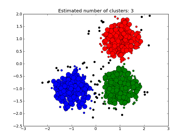
Density Based Clustering - DBSCAN
centers = [[1, 1], [-1, -1], [1, -1]]
X, labels_true = make_blobs(n_samples=750, centers=centers, cluster_std=0.4,random_state=0)
plt.scatter(X[:,0], X[:,1],s=10)
![]()
from sklearn.cluster import DBSCAN
from sklearn.preprocessing import StandardScaler
X = StandardScaler().fit_transform(X)db = DBSCAN(eps=0.3, min_samples=10).fit(X)
core_samples_mask = np.zeros_like(db.labels_, dtype=bool)
core_samples_mask[db.core_sample_indices_] = True
labels = db.labels_
plt.scatter(X[:,0], X[:,1],s=10,c=labels)
![]()
Measuring Performance of Clusters衡量聚类的性能
- Two forms of evaluation
- supervised, which uses a ground truth class values for each sample.
- completeness_score
- homogeneity_score
- unsupervised, which measures the quality of model itself
- silhoutte_score
- calinski_harabaz_score
- 两种评估形式
- 有监督的,它对每个样本使用基本事实类别值。
- completeness_score
- homogenity_score
- 无人监督,它衡量模型本身的质量
- silhoutte_score
- calinski_harabaz_score
completeness_score
- A clustering result satisfies completeness if all the data points that are members of a given class are elements of the same cluster.
- Accuracy is 1.0 if data belonging to same class belongs to same cluster, even if multiple classes belongs to same cluster
- 如果属于给定类的所有数据点都是同一群集的元素,则群集结果将满足完整性要求
- 如果属于同一类别的数据属于同一群集,则即使多个类别属于同一群集,精度也为1.0
from sklearn.metrics.cluster import completeness_scorecompleteness_score( labels_true=[10,10,11,11],labels_pred=[1,1,0,0])
1.0
- The acuracy is 1.0 because all the data belonging to same class belongs to same cluster
completeness_score( labels_true=[11,22,22,11],labels_pred=[1,0,1,1])
0.3836885465963443
- The accuracy is .3 because class 1 - [11,22,11], class 2 - [22]
print(completeness_score([10, 10, 11, 11], [0, 0, 0, 0]))
1.0
homogeneity_score
- A clustering result satisfies homogeneity if all of its clusters contain only data points which are members of a single class.
from sklearn.metrics.cluster import homogeneity_score
homogeneity_score([0, 0, 1, 1], [1, 1, 0, 0])
1.0
homogeneity_score([0, 0, 1, 1], [0, 1, 2, 3])
0.9999999999999999
homogeneity_score([0, 0, 0, 0], [1, 1, 0, 0])
1.0
- Same class data is broken into two clusters
silhoutte_score
- The Silhouette Coefficient is calculated using the mean intra-cluster distance (a) and the mean nearest-cluster distance (b) for each sample.
- The Silhouette Coefficient for a sample is (b - a) / max(a, b). To clarify, b is the distance between a sample and the nearest cluster that the sample is not a part of.
Example : Selecting the number of clusters with silhouette analysis on KMeans clustering
from sklearn.datasets import make_blobs
X, Y = make_blobs(n_samples=500,n_features=2,centers=4,cluster_std=1,center_box=(-10.0, 10.0),shuffle=True,random_state=1)
plt.scatter(X[:,0],X[:,1],s=10)
![]()
range_n_clusters = [2, 3, 4, 5, 6]
from sklearn.cluster import KMeans
from sklearn.metrics import silhouette_score
for n_cluster in range_n_clusters:kmeans = KMeans(n_clusters=n_cluster)kmeans.fit(X)labels = kmeans.predict(X)print (n_cluster, silhouette_score(X,labels))
2 0.7049787496083262
3 0.5882004012129721
4 0.6505186632729437
5 0.5745029081702377
6 0.4544511749648251
- Optimal number of clusters seems to be 2
calinski_harabaz_score
- The score is defined as ratio between the within-cluster dispersion and the between-cluster dispersion.
- 群集的最佳数量似乎是2
- 分数定义为群集内分散度和群集间分散度之间的比率。
from sklearn.metrics import calinski_harabaz_scorefor n_cluster in range_n_clusters:kmeans = KMeans(n_clusters=n_cluster)kmeans.fit(X)labels = kmeans.predict(X)print (n_cluster, calinski_harabaz_score(X,labels))
2 1604.112286409658
3 1809.991966958033
4 2704.4858735121097
5 2281.933655783649
6 2016.011232059114
python——聚类相关推荐
- python 聚类_使用python+sklearn实现聚类性能评估中随机分配对聚类度量值的影响
注意:单击此处https://urlify.cn/3iAzUr下载完整的示例代码,或通过Binder在浏览器中运行此示例 下图说明了聚类数量和样本数量对各种聚类性能评估度量指标的影响.未调整的度量指标 ...
- python 聚类算法包_Python聚类算法之DBSACN实例分析 python怎么用sklearn包进行聚类
python 怎么可视化聚类的结果 science 发表的聚类算法的python代码 测试数据长什...说明你的样本数据中有nan值,通常是因为原始数据中包含空字符串或None值引起的. 解决办法是把 ...
- python 聚类_聚类算法中的四种距离及其python实现
欧氏距离 欧式距离也就是欧几里得距离,是最常见也是最简单的一种距离,再n维空间下的公式为: 在python中,可以运用scipy.spatial.distance中的pdist方法来实现,但需要调整其 ...
- 10种Python聚类算法完整操作示例(建议收藏
来源:海豚数据科学实验室 著作权归作者所有,本文仅作学术分享,若侵权,请联系后台删文处理 !!文末附每日小知识点哦!! 聚类或聚类分析是无监督学习问题.它通常被用作数据分析技术,用于发现数据中的有趣模 ...
- Python聚类色彩提取——Scipy-kmeans
一.聚类:物以类聚 数组可以进行聚类,并找到数组的聚类中心.使用的第三方库是scipy,需要pip install scipy,先安装该库.数组聚类代码: import numpy as np fro ...
- python 散点图聚类,【聚类算法】10种Python聚类算法完整操作示例(建议收藏
点击上方,选择星标,每天给你送干货! 来源:海豚数据科学实验室著作权归作者所有,本文仅作学术分享,若侵权,请联系后台删文处理 聚类或聚类分析是无监督学习问题.它通常被用作数据分析技术,用于发现数据中的 ...
- python聚类算法中x是多维、y是一维怎么画图_基于Python的数据可视化:从一维到多维...
目录 一.iris数据集介绍 二.一维数据可视化 三.二维数据可视化 四.多维数据可视化 五.参考资料 一.iris数据集介绍 iris数据集有150个观测值和5个变量,分别是sepal length ...
- python聚类dbscan案例经纬度_用DBSCAN聚类经纬度坐标
用基于密度的聚类算法,计算坐标点聚集地,很好用. import pandas as pd import numpy as np from sklearn.cluster import DBSCAN f ...
- python聚类的结果显示_使用Python进行聚类
微信公众号:岭南见闻 关注可了解更多的数据处理技巧.问题或建议,请公众号留言; 如果你觉得文章对你有帮助,欢迎赞赏 导入数据,进行聚类from sklearn.datasets import load ...
最新文章
- 分享一段Java搞笑的代码注释
- 《Go语言从入门到实战》学习笔记(1)——Go语言学习路线图、简介
- 关于ASP.NET 中站点地图sitemap 的使用【转xugang】
- 怎么让用一行代码实现页面的定时强制刷新?脚本刷流量再也不用愁了!
- 32位机器下面各类型的取值范围(sizeof值)
- 如何在服务器运行aspx_ASP.NET开发实战——(四)MVC是如何运行?它的生命周期是什么?...
- 程序员应具备的素质[转帖]
- 流媒体压力测试工具—推拉流
- 在office2010的ppt中加入音乐
- okhttp的视频下载
- 【调试】——idea远程调试服务器上的代码
- 如何刷新本机DNS缓存(Win+Linux+OSX)
- c语言判断真假,C语言中的真假值
- matlab2012卸载,matlab2012一些函数删除后的替代解决方法及用到操作
- MATLAB图像融合拼接
- 视频融合平台EasyCVR集成播放器,但是无法播放该如何解决?
- 品牌连锁企业如何突破技术壁垒对接分账系统?
- 如果开了多个模拟器,那么如何知道每个模拟器对应的端口号
- 电销机器人价格_电话电销机器人价格如何?会很贵吗?
- 交流桩CP信号充电流程
热门文章
- 读《高效程序员的45个习惯——敏捷开发修炼之道》
- 好程序员web前端分享DIV+CSS3和html5+CSS3有什么区别
- 用树莓派做一个alibaba-guest
- android 发送http请求
- iPhone 6 Screens Demystified
- IOS学习笔记(九)之UIAlertView(警告视图)和UIActionSheet(操作表视图)基本概念和使用方法...
- 马虎的算式 - 蓝桥杯
- log4j 源码解析_log4j1.x设置自动加载log4j.xml
- linux 编译器错误,linux – GHCi – Haskell编译器错误 – /home/user/.ghci归其他人所有,IGNORING...
- 如何用node命令和webpack命令传递参数 转载