运动目标跟踪(四)--搜索算法优化搜索方向之Camshift
mean-shift 的特点是把支撑空间和特征空间在数据密度的框架下综合了起来。对图像来讲,支撑空间就是像素点的坐标,特征空间就是对应像素点的灰度或者RGB三分量。将这两个空间综合后,一个数据点就是一个5维的向量:[x,y,r,g,b]。
这在观念上看似简单,实质是一个飞跃,它是mean-shift方法的基点。
mean-shift方法很宝贵的一个特点就是在这样迭代计算的框架下,求得的mean-shift向量必收敛于数据密度的局部最大点。可以细看[ComaniciuMeer2002]的文章。
写了点程序,可以对图像做简单的mean-shift filtering,供参考:
%%%%%%%%%%%%%%%%%%%%%%%%%%%%%%%%%%%%%%
function [DRGB, DSD, MSSD] = MScut(sMode, RGB_raw, hs, hf, m );
% designed for segmenting a colour image using mean-shift [ComaniciuMeer 2002]
% image must be color
% procedure in mean-shift
% 1. combine support space and feature space to make a mean-shift space
% based data description
% 2. for every mean-shift space data
% 3. do mean-shift filtering
% until convergence
% 4. end
% 5. find the converged mean-shift space data that you are interested in
% and label it
% 6. repeat the above steps
%
% a -- data in support space
% b -- data in feature space
% x -- data in mean-shift space
% f(.) -- data density function
% k(.) -- profile function (implicit)
% g(.) -- profile function (explicit)
% m -- mean shift vector
% hs -- bandwidth in support space
% hf -- bandwidth in feature space
% M -- threshold to make a distinct cluster
%% enter $hs$, $hf$, $m$ if necessary
if ~exist('hs')
hs = input('please enter spatial bandwidth (hs):\n');
end
if ~exist('hf')
hf = input('please enter feature bandwidth (hf):\n');
end
if ~exist('m')
m = input('please enter minimum cluster size (m):\n');
end
switch upper(sMode)
case 'RGB'
RGB = double( RGB_raw );
case 'gray'
error('FCMcut must use colored image to do segmentation!')
end
sz = size(RGB);
mTCUT = Tcut( RGB(:,:,1) ); % trivial segmentation
%% project data into mean-shift space to make $MSSD$ (mean-shift space data)
mT = repmat([1:sz(1)]', 1, sz(2));
vX = mT(1:end)'; % row
mT = repmat([1:sz(2)], sz(1), 1);
vY = mT(1:end)'; % column
mT = RGB(:,:,1);
vR = mT(1:end)'; % red
mT = RGB(:,:,2);
vG = mT(1:end)'; % green
mT = RGB(:,:,3);
vB = mT(1:end)'; % blue
MSSD = [vX, vY, vR, vG, vB];
%% make $g$ - explicit profile function
disp('Using flat kernel: Epanechnikov kernel...')
g_s = ones(2*hs+1, 2); % 's' for support space
g_f = ones(2*hf+1, 3); % 'f' for feature space
%% main part $$
nIteration = 4;
nData = length(MSSD); % total number of data
DSD = MSSD*0; % 'DSD' for destination space data
for k = 1:nData
%
tMSSD = MSSD(k,:); % 't' for temp
for l = 1:nIteration
%
mT = abs( MSSD - repmat(tMSSD, nData, 1));
vT = logical( (mT(:,1)<=hs).*(mT(:,2)<=hs).*(mT(:,3)<=hf).*(mT(:,4)<=hf).*(mT(:,5)<=hf) );
v = MSSD(vT,:);
% update $tMSSD$
tMSSD = mean( v, 1 );
if nIteration == l
DSD(k,:) = tMSSD;
end
end
end
% show result
DRGB = RGB * 0;
DRGB(:,:,1) = reshape(DSD(:,3), sz(1), sz(2)); % red
DRGB(:,:,2) = reshape(DSD(:,4), sz(1), sz(2)); % red
DRGB(:,:,3) = reshape(DSD(:,5), sz(1), sz(2)); % red
figure, imshow(uint8(DRGB), [])
Mean shift算法的详细介绍,可以参见PAMI 2002的paper。
Comaniciu, D. and P. Meer (2002). "Mean shift: A robust approach toward feature space analysis." Pattern Analysis and Machine Intelligence, IEEE Transactions on 24(5): 603-619.
OpenCV分别实现了mean shift用来做跟踪、分割和滤波的函数。
其中滤波的c++函数原型为:
void pyrMeanShiftFiltering(InputArray src, OutputArray dst, double sp, double sr, intmaxLevel=1, TermCriteria termcrit=TermCriteria( TermCriteria::MAX_ITER+TermCriteria::EPS,5,1) )
src和dst分别为输入和输出图像,8 bit,3 channel,sp和sr为空间域和颜色域的半径,maxLevel为分割用金字塔的最大层数,termcrit为迭代的终止条件。
跟踪的函数原型为:
int meanShift(InputArray probImage, Rect& window, TermCriteria criteria)
proImage为生成的物体存在的概率图,window为初始化的搜索窗口(同时是输出的搜索结果),criteria为终止条件。
分割的函数原型为:
void gpu::meanShiftSegmentation(const GpuMat& src, Mat& dst, int sp, int sr, int minsize, TermCriteria criteria=TermCriteria(TermCriteria::MAX_ITER + TermCriteria::EPS, 5, 1))
大部分参数与pyrMeanShiftFiltering相同,minsize为最小的分割区域大小,小于这个大小的区域会被合并。
OpenCV sample里用pyrMeanShiftFiltering和floodfill函数共同实现了简单的分割的例子.(/samples/cpp/Meanshift_segmentation.cpp)。
Mean Shift算法,一般是指一个迭代的步骤,即先算出当前点的偏移均值,移动该点到其偏移均值,然后以此为新的起始点,继续移动,直到满足一定的条件结束.
1. Meanshift推导
给定d维空间Rd的n个样本点 ,i=1,…,n,在空间中任选一点x,那么Mean Shift向量的基本形式定义为:
![]()
![]()
![]()
![]()
![]()
把基本的meanshift向量加入核函数,核函数的性质在这篇博客介绍:http://www.cnblogs.com/liqizhou/archive/2012/05/11/2495788.html
解释一下K()核函数,h为半径,Ck,d/nhd 为单位密度,要使得上式f得到最大,最容易想到的就是对上式进行求导,的确meanshift就是对上式进行求导.![]()
![]()
K(x)叫做g(x)的影子核,名字听上去听深奥的,也就是求导的负方向,那么上式可以表示
![]()
![]()
![]()
上面介绍了meanshift的流程,但是比较散,下面具体给出它的算法流程。
2.meanshift在图像上的聚类:
一般一个图像就是个矩阵,像素点均匀的分布在图像上,就没有点的稠密性。所以怎样来定义点的概率密度,这才是最关键的。
如果我们就算点x的概率密度,采用的方法如下:以x为圆心,以h为半径。落在球内的点位xi 定义二个模式规则。
(1)x像素点的颜色与xi像素点颜色越相近,我们定义概率密度越高。
所以定义总的概率密度,是二个规则概率密度乘积的结果,可以(4)表示
![]()
其中:![]() 代表空间位置的信息,离远点越近,其值就越大,
代表空间位置的信息,离远点越近,其值就越大,![]() 表示颜色信息,颜色越相似,其值越大。如图左上角图片,按照(4)计算的概率密度如图右上。利用meanshift对其聚类,可得到左下角的图。
表示颜色信息,颜色越相似,其值越大。如图左上角图片,按照(4)计算的概率密度如图右上。利用meanshift对其聚类,可得到左下角的图。
|
|
|
|
|
|
camshift利用目标的颜色直方图模型将图像转换为颜色概率分布图,初始化一个搜索窗的大小和位置,并根据上一帧得到的结果自适应调整搜索窗口的位置和大小,从而定位出当前图像中目标的中心位置。
分为三个部分:
1--色彩投影图(反向投影):
(1).RGB颜色空间对光照亮度变化较为敏感,为了减少此变化对跟踪效果的影响,首先将图像从RGB空间转换到HSV空间。(2).然后对其中的H分量作直方图,在直方图中代表了不同H分量值出现的概率或者像素个数,就是说可以查找出H分量大小为h的概率或者像素个数,即得到了颜色概率查找表。(3).将图像中每个像素的值用其颜色出现的概率对替换,就得到了颜色概率分布图。这个过程就叫反向投影,颜色概率分布图是一个灰度图像。
2--meanshift
meanshift算法是一种密度函数梯度估计的非参数方法,通过迭代寻优找到概率分布的极值来定位目标。
算法过程为:
(1).在颜色概率分布图中选取搜索窗W
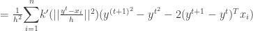
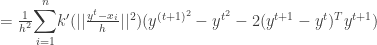
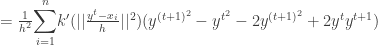
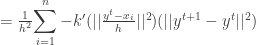
(2).计算零阶距:

计算一阶距:

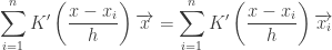
计算搜索窗的质心:

(3).调整搜索窗大小
宽度为 ;长度为1.2s;
(4).移动搜索窗的中心到质心,如果移动距离大于预设的固定阈值,则重复2)3)4),直到搜索窗的中心与质心间的移动距离小于预设的固定阈值,或者循环运算的次数达到某一最大值,停止计算。关于meanshift的收敛性证明可以google相关文献。
3--camshift
将meanshift算法扩展到连续图像序列,就是camshift算法。它将视频的所有帧做meanshift运算,并将上一帧的结果,即搜索窗的大小和中心,作为下一帧meanshift算法搜索窗的初始值。如此迭代下去,就可以实现对目标的跟踪。
算法过程为:
(1).初始化搜索窗
(2).计算搜索窗的颜色概率分布(反向投影)
(3).运行meanshift算法,获得搜索窗新的大小和位置。
(4).在下一帧视频图像中用(3)中的值重新初始化搜索窗的大小和位置,再跳转到(2)继续进行。
camshift能有效解决目标变形和遮挡的问题,对系统资源要求不高,时间复杂度低,在简单背景下能够取得良好的跟踪效果。但当背景较为复杂,或者有许多与目标颜色相似像素干扰的情况下,会导致跟踪失败。因为它单纯的考虑颜色直方图,忽略了目标的空间分布特性,所以这种情况下需加入对跟踪目标的预测算法。
Camshift的opencv实现
原文http://blog.csdn.net/houdy/archive/2004/11/10/175739.aspx
1--Back Projection
计算Back Projection的OpenCV代码。
(1).准备一张只包含被跟踪目标的图片,将色彩空间转化到HSI空间,获得其中的H分量:
IplImage* target=cvLoadImage("target.bmp",-1); //装载图片
IplImage* target_hsv=cvCreateImage( cvGetSize(target), IPL_DEPTH_8U, 3 );
IplImage* target_hue=cvCreateImage( cvGetSize(target), IPL_DEPTH_8U, 3 );
cvCvtColor(target,target_hsv,CV_BGR2HSV); //转化到HSV空间
cvSplit( target_hsv, target_hue, NULL, NULL, NULL ); //获得H分量
(2).计算H分量的直方图,即1D直方图:
IplImage* h_plane=cvCreateImage( cvGetSize(target_hsv),IPL_DEPTH_8U,1 );
int hist_size[]={255}; //将H分量的值量化到[0,255]
float* ranges[]={ {0,360} }; //H分量的取值范围是[0,360)
CvHistogram* hist=cvCreateHist(1, hist_size, ranges, 1);
cvCalcHist(&target_hue, hist, 0, NULL);
在这里需要考虑H分量的取值范围的问题,H分量的取值范围是[0,360),这个取值范围的值不能用一个byte来表示,为了能用一个byte表示,需要将H值做适当的量化处理,在这里我们将H分量的范围量化到[0,255]。
(3).计算Back Projection:
IplImage* rawImage;
//get from video frame,unsigned byte,one channel
IplImage* result=cvCreateImage(cvGetSize(rawImage),IPL_DEPTH_8U,1);
cvCalcBackProject(&rawImage,result,hist);
(4). result即为我们需要的.
2--Mean Shift算法
质心可以通过以下公式来计算:
(1).计算区域内0阶矩
for(int i=0;i< height;i++)
for(int j=0;j< width;j++)
M00+=I(i,j)
(2).区域内1阶矩:
for(int i=0;i< height;i++)
for(int j=0;j< width;j++)
{
M10+=i*I(i,j);
M01+=j*I(i,j);
}
(3).则Mass Center为:
Xc=M10/M00; Yc=M01/M00
在OpenCV中,提供Mean Shift算法的函数,函数的原型是:
int cvMeanShift(IplImage* imgprob,CvRect windowIn,
CvTermCriteria criteria,CvConnectedComp* out);
需要的参数为:
(1).IplImage* imgprob:2D概率分布图像,传入;
(2).CvRect windowIn:初始的窗口,传入;
(3).CvTermCriteria criteria:停止迭代的标准,传入;
(4).CvConnectedComp* out:查询结果,传出。
注:构造CvTermCriteria变量需要三个参数,一个是类型,另一个是迭代的最大次数,最后一个表示特定的阈值。例如可以这样构造 criteria:
criteria=cvTermCriteria(CV_TERMCRIT_ITER|CV_TERMCRIT_EPS,10,0.1)。
3--CamShift算法
整个算法的具体步骤分5步:
Step 1:将整个图像设为搜寻区域。
Step 2:初始话Search Window的大小和位置。
Step 3:计算Search Window内的彩色概率分布,此区域的大小比Search Window要稍微大一点。
Step 4:运行MeanShift。获得Search Window新的位置和大小。
Step 5:在下一帧视频图像中,用Step 3获得的值初始化Search Window的位置和大小。跳转到Step 3继续运行。
OpenCV代码:
在OpenCV中,有实现CamShift算法的函数,此函数的原型是:
cvCamShift(IplImage* imgprob, CvRect windowIn,
CvTermCriteria criteria,
CvConnectedComp* out, CvBox2D* box=0);
其中:
imgprob:色彩概率分布图像。
windowIn:Search Window的初始值。
Criteria:用来判断搜寻是否停止的一个标准。
out:保存运算结果,包括新的Search Window的位置和面积。
box:包含被跟踪物体的最小矩形。
更多参考:
带有注释的camshift算法的opencv实现代码见:
http://download.csdn.net/source/1663015
Introduction To Mean Shift Algorithm
http://saravananthirumuruganathan.wordpress.com/2010/04/01/introduction-to-mean-shift-algorithm/
Its been quite some time since I wrote a Data Mining post . Today, I intend to post on Mean Shift – a really cool but not very well known algorithm. The basic idea is quite simple but the results are amazing. It was invented long back in 1975 but was not widely used till two papers applied the algorithm to Computer Vision.
I learned this algorithm in my Advanced Data Mining course and I wrote the lecture notes on it. So here I am trying to convert my lecture notes to a post. I have tried to simplify it – but this post is quite involved than the other posts.
It is quite sad that there exists no good post on such a good algorithm. While writing my lecture notes, I struggled a lot for good resources ![]() . The 3 “classic" papers on Mean Shift are quite hard to understand. Most of the other resources are usually from Computer Vision courses where Mean Shift is taught lightly as yet another technique for vision tasks (like segmentation) and contains only the main intuition and the formulas.
. The 3 “classic" papers on Mean Shift are quite hard to understand. Most of the other resources are usually from Computer Vision courses where Mean Shift is taught lightly as yet another technique for vision tasks (like segmentation) and contains only the main intuition and the formulas.
As a disclaimer, there might be errors in my exposition – so if you find anything wrong please let me know and I will fix it. You can always check out the reference for more details. I have not included any graphics in it but you can check the ppt given in the references for an animation of Mean Shift.
Introduction
Intuitive Idea of Mean Shift
Preliminaries
Kernels :
A kernel is a function that satisfies the following requirements :


Some examples of kernels include :


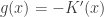
Gradient Ascent Nature of Mean Shift

Applying it to kernel density estimator,


Mean Shift
 , we have
 is called as the mean shift. So mean shift procedure can be summarized as : For each point

2. Move the density estimation window by
Using a Gaussian kernel as an example,


Proof Of Convergence

To prove the convergence , we have to prove that
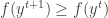
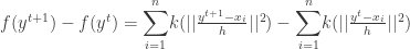
But since the kernel is a convex function we have ,


 is convergent. The second part of the proof in [2] which tries to prove the sequence
  is convergent is wrong.
Improvements to Classic Mean Shift Algorithm
 where
where  is the number of iterations and
  is the number of data points in the data set. Many improvements have been made to the mean shift algorithm to make it converge faster.
 parameter is calculated using kNN algorithm. If
  is the k-nearest neighbor of
Here we use 


Other Issues
Applications of Mean Shift
Comparison with K-Means
 where k is the number of clusters, n is the number of points and T is the number of iterations. Classic mean shift is computationally expensive with a time complexity
 References
运动目标跟踪(四)--搜索算法优化搜索方向之Camshift相关推荐
- 运动目标跟踪(三)--搜索算法优化搜索方向之Meanshift
原文: http://blog.csdn.net/jinshengtao/article/details/30258833 这次将介绍基于MeanShift的目标跟踪算法,首先谈谈简介,然后给出算法实 ...
- OpenCV学习笔记(三十六)——Kalman滤波做运动目标跟踪 OpenCV学习笔记(三十七)——实用函数、系统函数、宏core OpenCV学习笔记(三十八)——显示当前FPS OpenC
OpenCV学习笔记(三十六)--Kalman滤波做运动目标跟踪 kalman滤波大家都很熟悉,其基本思想就是先不考虑输入信号和观测噪声的影响,得到状态变量和输出信号的估计值,再用输出信号的估计误差加 ...
- 基于MATLAB的视频运动目标跟踪与检测定位系统
一.课题背景 视频运动目标检测与跟踪算法是计算机视觉领域的一个核心课题,也是智能视频监控系统的关键底层技术.它融合了图像处理.人工智能等领域的研究成果,已经广泛应用于安保监控.智能武器.视频会议.视频 ...
- 运动目标跟踪算法综述
运动目标跟踪是视频监控系统中不可缺少的环节.在特定的场景中,有一些经典的算法可以实现比较好的目标跟踪效果.本文介绍了一般的目标跟踪算法,对几个常用的算法进行对比,并详细介绍了粒子滤波算法和基于轮廓的目 ...
- OpenCV学习笔记(二十六)——小试SVM算法ml OpenCV学习笔记(二十七)——基于级联分类器的目标检测objdect OpenCV学习笔记(二十八)——光流法对运动目标跟踪Video Ope
OpenCV学习笔记(二十六)--小试SVM算法ml 总感觉自己停留在码农的初级阶段,要想更上一层,就得静下心来,好好研究一下算法的东西.OpenCV作为一个计算机视觉的开源库,肯定不会只停留在数字图 ...
- linux 内核连接跟踪,Linux内核连接跟踪锁的优化分析(1)
Linux内核连接跟踪锁的优化分析(1) 作者:gfree.wind@gmail.com 博客:linuxfocus.blog.chinaunix.net 微博:weibo.com/glinuxer ...
- 随机数字信号处理期末大报告——基于卡尔曼滤波的自由落体运动目标跟踪MATLAB实现
完整的实验报告下载随机数字信号处理期末大报告-基于卡尔曼滤波的自由落体运动目标跟踪.docx-机器学习文档类资源-CSDN下载 程序包及所需数据下载 target tracking us ...
- Kalman 滤波用于自由落体运动目标跟踪问题
某一物体在重力场做自由落体运动.观测装置对其位移进行检测,在传感器受到未知的独立分布随机信号的干扰下,我们需要估计该物体的运动位移和速度,该系统是二维状态估计系统. 不考虑x方向上位置变化,只估计y轴 ...
- MATLAB实现基于遗传算法/引力搜索算法优化新安江水文模型
MATLAB实现基于遗传算法/引力搜索算法优化新安江水文模型 1 新安江模型 1.1 新安江模型结构 1.2 模型参数种类及意义 2 新安江模型优化参数 2.1 蒸散发参数: KC.WUM.WLM.C ...
最新文章
- 在列表显示某个内容,但数据表没有这个字段
- html判断数字数据的大小写,判断一个字符是否是数字、还是大小写字母
- debian/ubuntu下安装java8
- OAuth2.0学习(1-6)授权方式3-密码模式(Resource Owner Password Credentials Grant)
- 编程的首要原则(s)是什么?
- PAT_B_1035_Java(25分)
- dask 使用_在Google Cloud上使用Dask进行可扩展的机器学习
- 吃冰淇淋更容易溺水?
- meta http-equiv=X-UA-Compatible content=IE=edge / 的说明
- 如何在手机上打开xmind文件_xmind在手机上怎么操作
- 学生管理系统--golang--简单版本---开发框架
- Windows 10家庭版和专业版的区别在哪?Windows 10专业版好还是家庭版好?
- win10没有android驱动安装,win10系统安装adb驱动的详细步骤
- 苹果计算机重装系统步骤,苹果笔记本电脑重装mac系统教程
- 中国家庭追踪调查(CFPS)数据及问卷(2010-2018年)
- day42.自动关机小程序
- Objective-C学习笔记(1)——OC的基本概念和类
- 沈阳市中考计算机考试时间,2021辽宁沈阳中考考试时间、科目分值及时间轴
- 如何实现 “中间这几个字要加粗,但是不要太粗,比较纤细的那种粗” ?
- 【PAT A1094】The Largest Generation