R软件学习笔记-5（R软件画图）

转自：http://www.dataguru.cn/article-2421-1.html

摘要: 一、直方图绘制直方图函数：hist()对x1进行直方图分析 hist(x$x1)二、散点图散点图绘制函数：plot()探索各科成绩的关联关系 plot(x1,x2) plot(x$x1,x$x2)三、柱状图列联表分析列联函数table()：统计每个分数的人 ...

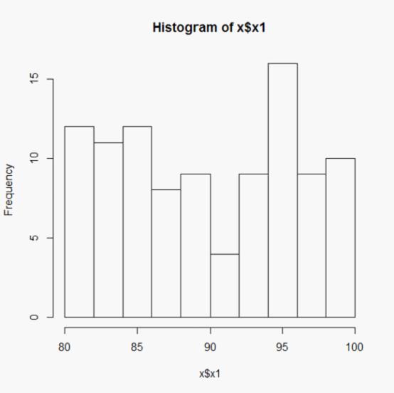
一、直方图

绘制直方图函数：hist()

对x1进行直方图分析

> hist(x$x1)>

二、散点图

散点图绘制函数：plot()

探索各科成绩的关联关系

> plot(x1,x2)> plot(x$x1,x$x2)>

三、柱状图

列联表分析

列联函数table()：统计每个分数的人数;

柱状图绘制函数：barplot()

> table(x$x1)  80  81  82  83  84  85  86  87  88  89  90  91  92  93  94  95  96  97  98  1   5   6   6   5   7   5   6   2   3   6   2   2   5   4  11   5   4   5 99 100  8   2> barplot(table(x$x1))>

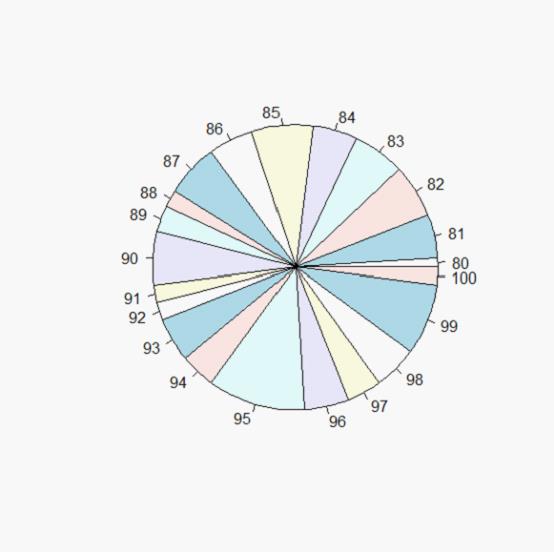
四、饼图

饼图绘制函数：pie()

> pie(table(x$x1))>

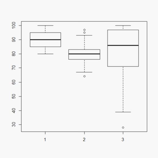
五、箱尾图

1、箱尾图绘制函数：boxplot()

> boxplot(x$x1,x$x2,x$x3)>

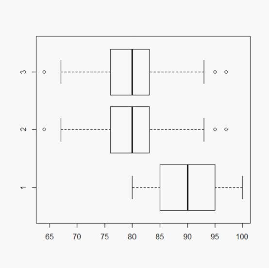
(1) 箱子的上下横线为样本的25%和75%分位数
(2) 箱子中间的横线为样本的中位数
(3) 上下延伸的直线称为尾线，尾线的
(4) 尽头为最高值和最低值
(5) 异常值

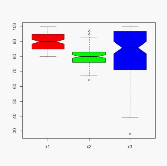
2、为箱尾图添加颜色和缺口

添加参数：颜色 col=c(c(“red”,”green”,”blue”))；缺口：notch=T。

> boxplot(x[2:4],col=c("red","green","blue"),notch=T)>

3、水平放置的箱尾图

添加参数：horizontal=T

> boxplot(x$x1,x$x2,x$x2,horizontal=T)>

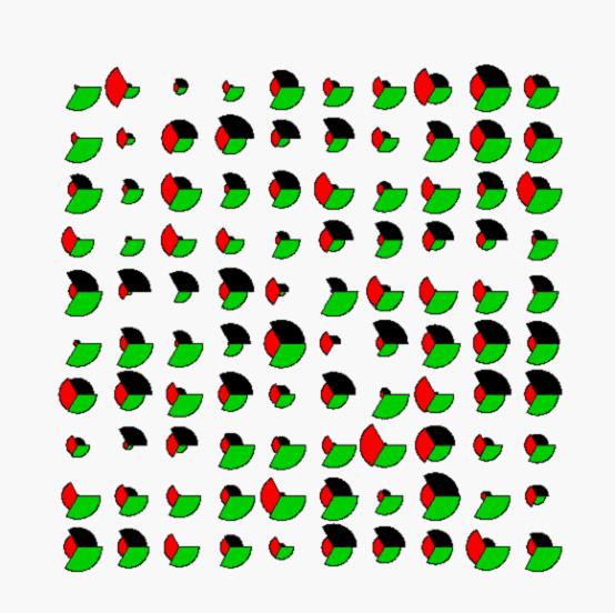
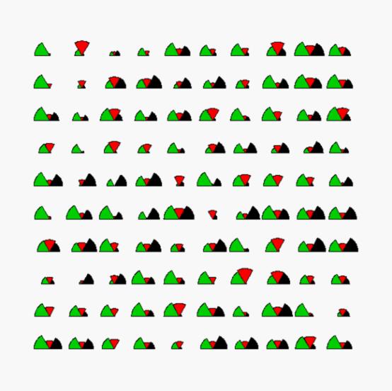
六、星相图

函数：stars()

1、

> stars(x[c("x1","x2","x3")])>

(1) 每个观测单位的数值表示为一个图形
(2) 每个图的每个角表示一个变量，字符串类型会标注在图的下方
(3) 角线的长度表达值的大小

2、扇形图 (雷达图)

添加参数：draw.segment=T 控制是否画扇形；full=T 控制是圆还是半圆。

> stars(x[c("x1","x2","x3")],full=T,draw.segment=T)>

扇形的面积越大，表示值越大。

3、半扇形

> stars(x[c("x1","x2","x3")],full=F,draw.segment=T)>

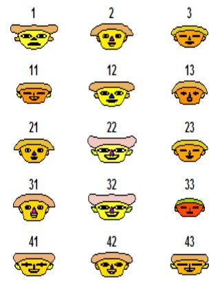
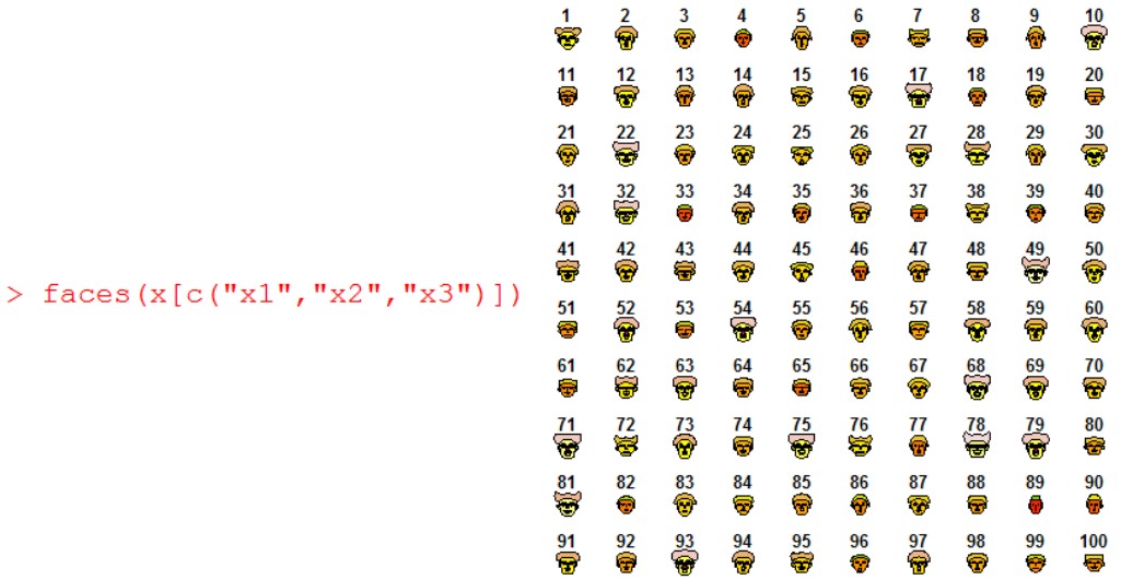
七、脸谱图

1、安装aplpack包

(1) 用五官的宽度和高度来描绘数值
(2) 人对脸谱高度敏感和强记忆
(3) 适合较少样本的情况

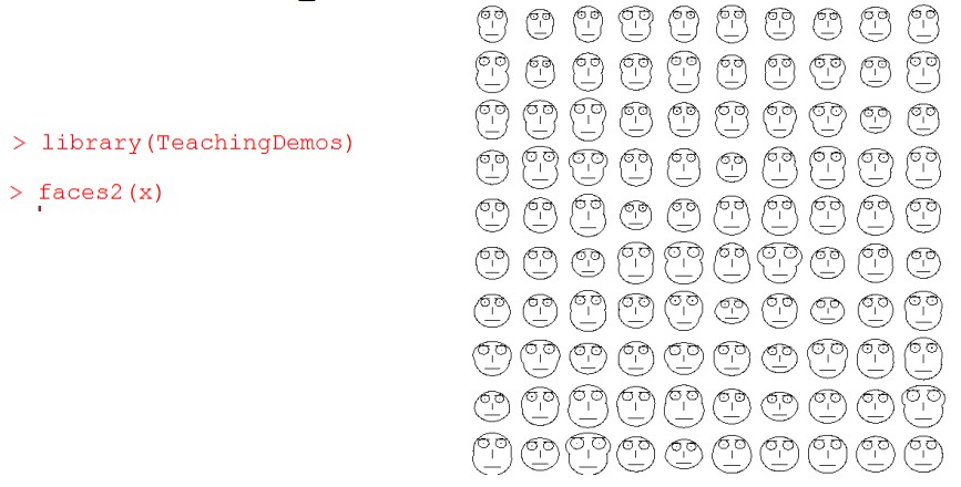
2、其他脸谱图

安装TeachingDemos包

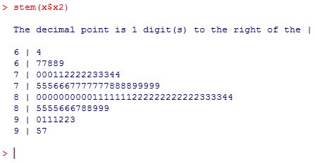
八、茎叶图

绘制茎叶图函数：stem()

> stem(x$x2)   The decimal point is 1 digit(s) to the right of the |   6 | 4  6 | 77889  7 | 000112222233344  7 | 5556667777777888899999  8 | 00000000001111111222222222222333344  8 | 5555666788999  9 | 0111223  9 | 57 >

上面茎叶图中：6 | 4 ，表示64分的有一个；6 | 77889 ，表示67分有两位同学，68分的有两位同学，69分的有一位同学。后面以此类推。

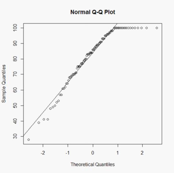
九、QQ图

函数：qqnorm(),qqline()

(1) 可用于判断是否正态分布
(2) 直线的斜率是标准差，截距是均值
(3) 点的散布越接近直线，则越接近正态分布

> qqnorm(x3)> qqline(x3)>

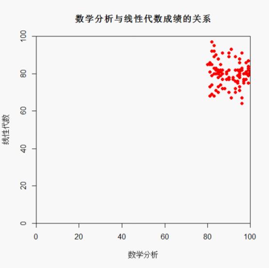
十、散点图的进一步设置

1、 plot(x$x1,x$x2,
main=”数学分析与线性代数成绩的关系”,
xlab=”数学分析”,
ylab=”线性代数”,
xlim=c(0,100),
ylim=c(0,100),
xaxs=”i”, #Set x axis style as internal
yaxs=”i”, #Set y axis style as internal
col=”red”, #Set the color of plotting symbol to r
pch=19) #Set the plotting symbol to filled dots

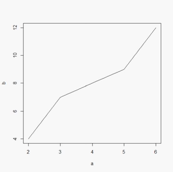
2、连线图

添加参数：type=”l”

> a=c(2,3,4,5,6)> b=c(4,7,8,9,12)> plot(a,b,type="l")>

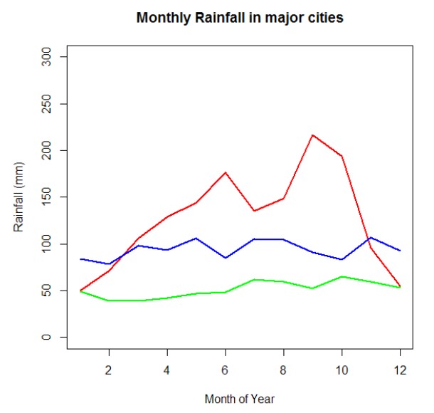
3、多条曲线的效果

plot(rain$Tokyo,type=”l”,col=”red”,
ylim=c(0,300),
main=”Monthly Rainfall in major cities”,
xlab=”Month of Year”,
ylab=”Rainfall (mm)”,
lwd=2 #线框大小粗细)
lines(rain$NewYork,type=”l”,col=”blue”,lwd=2)
lines(rain$London,type=”l”,col=”green”,lwd=2)
lines(rain$Berlin,type=”l”,col=”orange”,lwd=2)

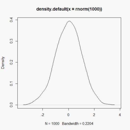
十一、密度图

函数：density()

> plot(density(rnorm(1000)))>

十二、热力图

1、R内置的数据集，使用函数data()列出。

> data()> mtcars                     mpg cyl  disp  hp drat    wt  qsec vs am gear carbMazda RX4           21.0   6 160.0 110 3.90 2.620 16.46  0  1    4    4Mazda RX4 Wag       21.0   6 160.0 110 3.90 2.875 17.02  0  1    4    4Datsun 710          22.8   4 108.0  93 3.85 2.320 18.61  1  1    4    1Hornet 4 Drive      21.4   6 258.0 110 3.08 3.215 19.44  1  0    3    1Hornet Sportabout   18.7   8 360.0 175 3.15 3.440 17.02  0  0    3    2Valiant             18.1   6 225.0 105 2.76 3.460 20.22  1  0    3    1Duster 360          14.3   8 360.0 245 3.21 3.570 15.84  0  0    3    4Merc 240D           24.4   4 146.7  62 3.69 3.190 20.00  1  0    4    2Merc 230            22.8   4 140.8  95 3.92 3.150 22.90  1  0    4    2Merc 280            19.2   6 167.6 123 3.92 3.440 18.30  1  0    4    4Merc 280C           17.8   6 167.6 123 3.92 3.440 18.90  1  0    4    4Merc 450SE          16.4   8 275.8 180 3.07 4.070 17.40  0  0    3    3Merc 450SL          17.3   8 275.8 180 3.07 3.730 17.60  0  0    3    3Merc 450SLC         15.2   8 275.8 180 3.07 3.780 18.00  0  0    3    3Cadillac Fleetwood  10.4   8 472.0 205 2.93 5.250 17.98  0  0    3    4Lincoln Continental 10.4   8 460.0 215 3.00 5.424 17.82  0  0    3    4Chrysler Imperial   14.7   8 440.0 230 3.23 5.345 17.42  0  0    3    4Fiat 128            32.4   4  78.7  66 4.08 2.200 19.47  1  1    4    1Honda Civic         30.4   4  75.7  52 4.93 1.615 18.52  1  1    4    2Toyota Corolla      33.9   4  71.1  65 4.22 1.835 19.90  1  1    4    1Toyota Corona       21.5   4 120.1  97 3.70 2.465 20.01  1  0    3    1Dodge Challenger    15.5   8 318.0 150 2.76 3.520 16.87  0  0    3    2AMC Javelin         15.2   8 304.0 150 3.15 3.435 17.30  0  0    3    2Camaro Z28          13.3   8 350.0 245 3.73 3.840 15.41  0  0    3    4Pontiac Firebird    19.2   8 400.0 175 3.08 3.845 17.05  0  0    3    2Fiat X1-9           27.3   4  79.0  66 4.08 1.935 18.90  1  1    4    1Porsche 914-2       26.0   4 120.3  91 4.43 2.140 16.70  0  1    5    2Lotus Europa        30.4   4  95.1 113 3.77 1.513 16.90  1  1    5    2Ford Pantera L      15.8   8 351.0 264 4.22 3.170 14.50  0  1    5    4Ferrari Dino        19.7   6 145.0 175 3.62 2.770 15.50  0  1    5    6Maserati Bora       15.0   8 301.0 335 3.54 3.570 14.60  0  1    5    8Volvo 142E          21.4   4 121.0 109 4.11 2.780 18.60  1  1    4    2>

2、利用内置的mtcars数据集绘制

首先要将数据框转换为矩阵。颜色越深，数值越大。

heatmap(as.matrix(mtcars),
Rowv=NA,
Colv=NA,
col = heat.colors(256),
scale=”column”,
margins=c(2,8),
main = “Car characteristics by
Model”)

十三、向日葵散点图

1、Iris(鸢尾花)数据集

2、向日葵散点图

函数：sunflowerplot()，参数col设定点的颜色，seg.col设定点发出的射线(代表重合点)的颜色。

(1) 用来克服散点图中数据点重叠问题
(2) 在有重叠的地方用一朵“向日葵花”的花瓣数目来表示重叠数据的个数

> sunflowerplot(iris[,3:4],col="gold",seg.col="gold")>

十四、散点图集

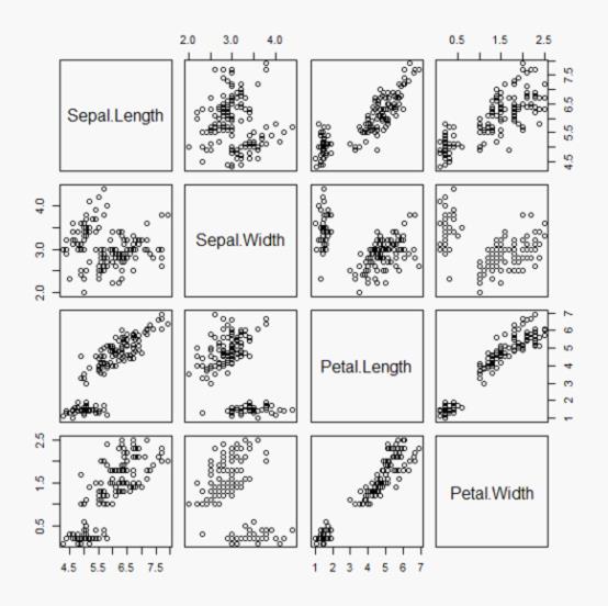
1、使用函数pairs()

(1) 遍历样本中全部的变量配对画出二元图
(2) 直观地了解所有变量之间的关系

> pairs(iris[,1:4])>

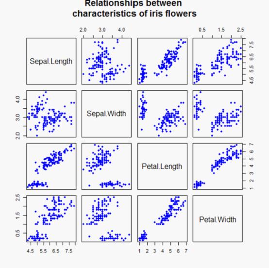
2、使用plot()函数

plot(iris[,1:4],
main=”Relationships between
characteristics of iris flowers”,
pch=19,
col=”blue”,
cex=0.9)

3、使用par()函数设置

(1) 利用par( )在同一个device输出多个散点图
(2) Par命令博大精深，用于设置绘图参数，help(par)

par(mfrow=c(3,1)) #在一张device中显示3行一列的图形
plot(x1,x2);plot(x2,x3);plot(x3,x1)

十五、关于绘图参数

1、寻求帮助

(1) help(par)
(2) 有哪些颜色？使用函数 colors()

2、绘图设备

dev.cur()
dev.list()
dev.next(which = dev.cur())
dev.prev(which = dev.cur())
dev.off(which = dev.cur())
dev.set(which = dev.next())
dev.new(…)
graphics.off()

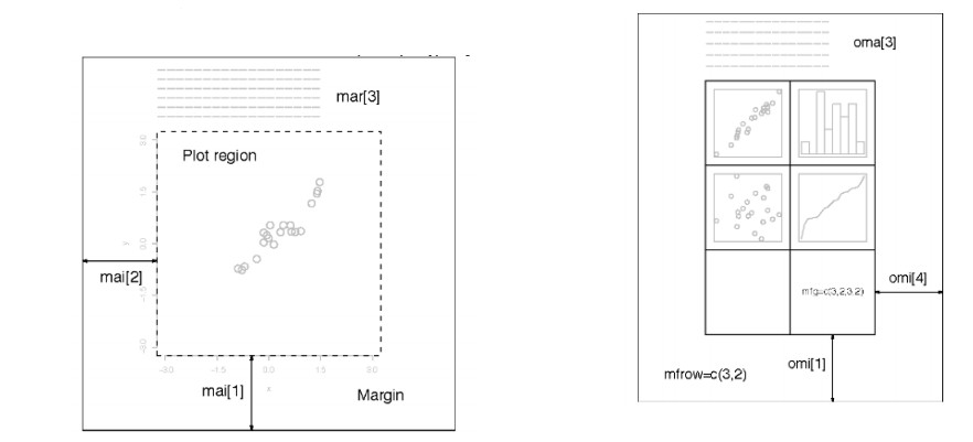
3、位置控制参数

(1) mai参数：A numerical vector of the form c(bottom, left, top, right) which gives the margin size specified in inches.

(2) oma参数：A vector of the form c(bottom, left, top, right) giving the size of the outer margins in lines of text.

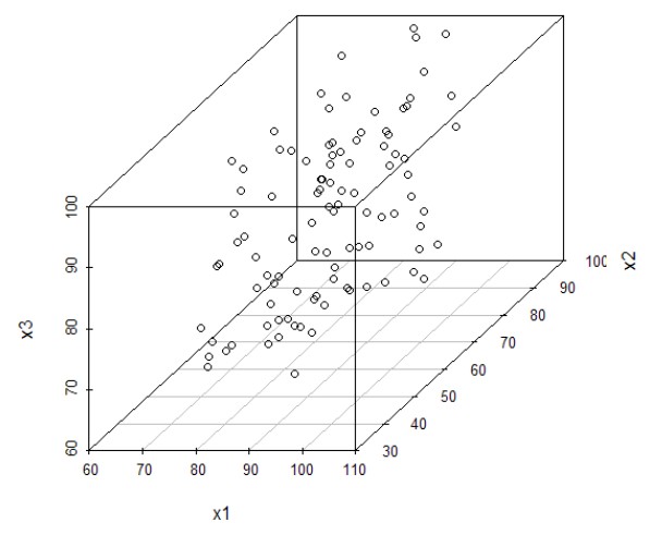
十六、三维散点图

安装scatterplot3d 包

scatterplot3d(x[2:4])

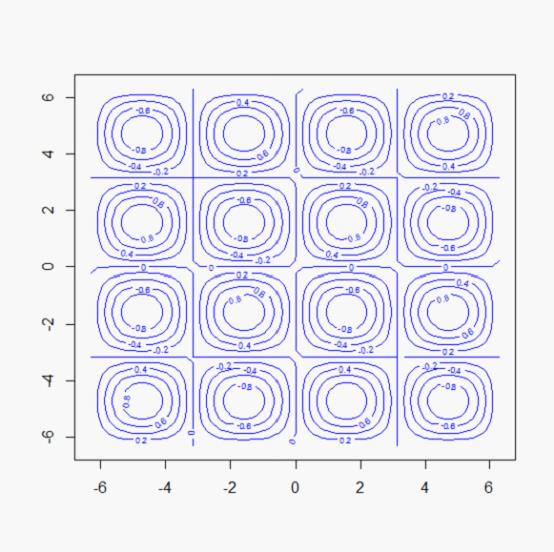
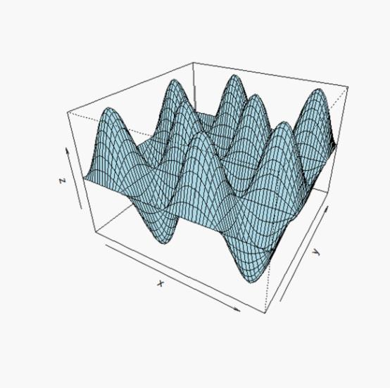
十七、三维作图

x<-y<-seq(-2*pi, 2*pi, pi/15)
f<-function(x,y) sin(x)*sin(y)
z<-outer(x, y, f)
contour(x,y,z,col="blue")
persp(x,y,z,theta=30, phi=30,expand=0.7,col="lightblue")

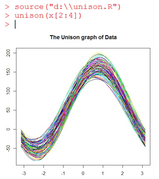
十八、调和曲线图

调和曲线用于聚类判断非常方便。

自定义函数unison的脚本unison.r：

unison<-function(x){   # x is a matrix or data frame of data   if (is.data.frame(x)==TRUE)      x<-as.matrix(x)   t<-seq(-pi, pi, pi/30)   m<-nrow(x); n<-ncol(x)   f<-array(0, c(m,length(t)))   for(i in 1:m){      f[i,]<-x[i,1]/sqrt(2)      for( j in 2:n){          if (j%%2==0)             f[i,]<-f[i,]+x[i,j]*sin(j/2*t)          else             f[i,]<-f[i,]+x[i,j]*cos(j%/%2*t)      }   }   plot(c(-pi,pi), c(min(f),max(f)), type="n",        main="The Unison graph of Data",        xlab="t", ylab="f(t)")  for(i in 1:m) lines(t, f[i,] , col=i)}

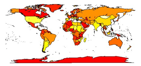
十九、地图

安装maps包

map(“state”, interior = FALSE)

map(“state”, boundary = FALSE, col=”red”,add = TRUE)
map(‘world’, fill = TRUE,col=heat.colors(10))

相关R绘图书籍：《R Graphs Cookbook》

R软件学习笔记-5（R软件画图）相关推荐

[R语言学习笔记1] R语言for循环的使用
学习R语言的过程中,后期逐渐就会用循环语句来减少自己的重复工作.所以了解for循环,是必备技能之一. R语言中的for循环结构是: for (循环变量 in 序列向量){表达式1表达式2...} 要注 ...
R语言学习笔记--《R语言实战》
文章目录 R语言基础一.数据结构 1. 向量 2. 矩阵 3. 数组 4. 数据框 5.列表二.数据输入 1.键盘输入 2.分隔符文本输入 (csv) 图形初阶一.图形参数 1.符号和线条 2. ...
r语言绘制精美pcoa图_[R语言学习笔记]用R做主坐标分析（PCoA）
原始数据为遗传距离矩阵,使用ape包的pcoa函数进行主坐标分析,然后使用ggplot2进行绘图. 欢迎大家批评指正转载请标明出处:https://www.ivistang.com/articles ...
R语言学习笔记（1~3）
R语言学习笔记(1~3) 一.R语言介绍 x <- rnorm(5) 创建了一个名为x的向量对象,它包含5个来自标准正态分布的随机偏差. 1.1 注释由符号#开头. #函数c()以向量的形式输 ...
R语言学习笔记——入门篇：第一章-R语言介绍
R语言 R语言学习笔记--入门篇:第一章-R语言介绍文章目录 R语言一.R语言简介 1.1.R语言的应用方向 1.2.R语言的特点二.R软件的安装 2.1.Windows/Mac 2.2.Lin ...
InSAR学习笔记之ISCE 软件安装
InSAR学习笔记之ISCE 软件安装 ISCE是一款常用的InSAR数据处理软件,2018年更新的版本基于ubuntu18.04系统安装过程简化了很多,本文分享一下安装过程.(之前在ubuntu16 ...
R语言学习笔记——入门篇：第三章-图形初阶
R语言 R语言学习笔记--入门篇:第三章-图形初阶文章目录 R语言一.使用图形 1.1.基础绘图函数:plot( ) 1.2.图形控制函数:dev( ) 补充--直方图函数:hist( ) 补充- ...
R语言学习笔记 06 岭回归、lasso回归
R语言学习笔记文章目录 R语言学习笔记比较lm.ridge和glmnet函数画岭迹图图6-4 <统计学习导论基于R语言的应用>P182 图6-6<统计学习导论基于R语言的 ...
r语言c函数怎么用,R语言学习笔记——C#中如何使用R语言setwd()函数
在R语言编译器中,设置当前工作文件夹可以用setwd()函数. > setwd("e://桌面//") > setwd("e:\桌面\") > ...
R语言学习笔记 07 Probit、Logistic回归
R语言学习笔记文章目录 R语言学习笔记 probit回归 factor()和as.factor() relevel() 案例11.4复刻 glm函数整理变量回归:Logistic和Probit- ...

R软件学习笔记-5（R软件画图）

R软件学习笔记-5（R软件画图）相关推荐

最新文章

热门文章