介绍 (Introduction)

What is Edge (or Fog) Computing?

什么是边缘(或雾)计算？

Gartner defines edge computing as: “a part of a distributed computing topology in which information processing is located close to the edge — where things and people produce or consume that information.”

Gartner将边缘计算定义为：“分布式计算拓扑的一部分，其中信息处理位于边缘附近-事物和人在此处生成或消费该信息。”

In other words, edge computing brings computation (and some data storage) closer to the devices where it’s data are being generated or consumed (especially in real-time), rather than relying on a cloud-based central system far away. With this approach, data does not suffer latency issues, reducing the amount of cost in transmission and processing. In a way, it is a kind of “return to the recent past,” where all the computational work was done locally on a desktop and not in the cloud.

换句话说，边缘计算使计算(和一些数据存储)更靠近要生成或使用其数据(特别是实时)的设备，而不是依赖于遥远的基于云的中央系统。 使用这种方法，数据不会出现延迟问题，从而减少了传输和处理的成本。 从某种意义上说，这是一种“回到最近的过去”，其中所有计算工作都在桌面上而不是在云中本地完成。

Edge computing was developed due to the exponential growth of IoT devices connected to the internet for either receiving information from the cloud or delivering data back to the cloud. And many Internet of Things (IoT) devices generate enormous amounts of data during their operations.

边缘计算的开发是由于连接到Internet的IoT设备呈指数级增长，以便从云中接收信息或将数据传递回云中。 许多物联网(IoT)设备在其运行期间会生成大量数据。

Edge computing provides new possibilities in IoT applications, particularly for those relying on machine learning (ML) for tasks such as object and pose detection, image (and face) recognition, language processing, and obstacle avoidance. Image data is an excellent addition to IoT, but also a significant resource consumer (as power, memory, and processing). Image processing “at the Edge”, running classics AI/ML models, is a great leap!

边缘计算为物联网应用提供了新的可能性，尤其是对于那些依靠机器学习(ML)完成诸如对象和姿态检测，图像(和面部)识别，语言处理以及避障等任务的应用。 图像数据是IoT的绝佳补充，同时也是重要的资源消耗者(如电源，内存和处理)。 运行经典AI / ML模型的“边缘”图像处理是一个巨大的飞跃！

Tensorflow Lite-机器学习(ML)处于边缘!! (Tensorflow Lite - Machine Learning (ML) at the edge!!)

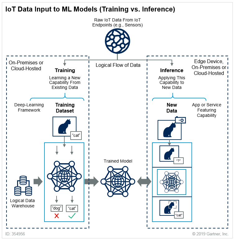
Machine Learning can be divided into two separated process: Training and Inference, as explained in Gartner Blog:

机器学习可以分为两个独立的过程：训练和推理，如Gartner Blog中所述 ：

• Training: Training refers to the process of creating a machine learning algorithm. Training involves using a deep-learning framework (e.g., TensorFlow) and training dataset (see the left-hand side of the above figure). IoT data provides a source of training data that data scientists and engineers can use to train machine learning models for various cases, from failure detection to consumer intelligence.

  培训：培训是指创建机器学习算法的过程。 培训涉及使用深度学习框架(例如TensorFlow)和培训数据集(请参见上图的左侧)。 物联网数据提供了训练数据的来源，数据科学家和工程师可以使用该数据来训练从故障检测到消费者智能的各种情况下的机器学习模型。

• Inference: Inference refers to the process of using a trained machine-learning algorithm to make a prediction. IoT data can be used as the input to a trained machine learning model, enabling predictions that can guide decision logic on the device, at the edge gateway, or elsewhere in the IoT system (see the right-hand side of the above figure).

  推论：推论是指使用经过训练的机器学习算法进行预测的过程。 IoT数据可以用作训练有素的机器学习模型的输入，从而启用可以指导设备，边缘网关或IoT系统中其他位置的决策逻辑的预测(请参见上图的右侧)。

TensorFlow Lite is an open-source deep learning framework that enables on-device machine learning inference with low latency and small binary size. It is designed to make it easy to perform machine learning on devices, “at the edge” of the network, instead of sending data back and forth from a server.

TensorFlow Lite是一个开源深度学习框架，可实现低延迟和小二进制大小的设备上机器学习推理 。 它旨在简化在“网络边缘”的设备上执行机器学习的过程，而不是从服务器来回发送数据。

Performing machine learning on-device can help to improve:

在设备上执行机器学习可以帮助改善：

• Latency: there’s no round-trip to a server

  延迟：服务器之间没有往返

• Privacy: no data needs to leave the device

  隐私权：无需任何数据即可离开设备

• Connectivity: an Internet connection isn’t required

  连接性：不需要Internet连接

• Power consumption: network connections are power-hungry

  功耗：网络连接耗电

TensorFlow Lite (TFLite) consists of two main components:

TensorFlow Lite(TFLite)包含两个主要组件：

• The TFLite converter, which converts TensorFlow models into an efficient form for use by the interpreter, and can introduce optimizations to improve binary size and performance.

  TFLite转换器将TensorFlow模型转换为供解释器使用的有效形式，并且可以引入优化以改善二进制大小和性能。

• The TFLite interpreter runs with specially optimized models on many different hardware types, including mobile phones, embedded Linux devices, and microcontrollers.

  TFLite解释器在许多不同的硬件类型(包括移动电话，嵌入式Linux设备和微控制器)上以经过特殊优化的模型运行。

In summary, a trained and saved TensorFlow model (like model.h5) can be converted using TFLite Converter in a TFLite FlatBuffer (like model.tflite) that will be used by TF Lite Interpreter inside the Edge device (as a Raspberry Pi), to perform inference on a new data.

总之，可以在TFLite FlatBuffer(例如model.tflite )中使用TFLite Converter转换经过训练并保存的TensorFlow模型(例如model.h5 )，该工具将由Edge设备(作为Raspberry Pi)中的TF Lite Interpreter使用，对新数据进行推断。

For example, I trained from scratch a simple CNN Image Classification model in my Mac (the “Server” on the above figure). The final model had 225,610 parameters to be trained, using as input the CIFAR10 dataset: 60,000 images (shape: 32, 32, 3). The trained model (cifar10_model.h5) had a size of 2.7Mb. Using the TFLite Converter, the model used on Raspberry Pi (model_cifar10.tflite) became with 905Kb (around 1/3 of original size). Making inference with both models (.h5 at Mac and .tflite at RPi) leaves the same results. Both notebooks can be found at GitHub.

例如，我从头开始在Mac中训练了一个简单的CNN图像分类模型(上图为“服务器”)。 最终模型具有225,610个要训练的参数，使用CIFAR10数据集作为输入：60,000张图像(形状：32、32、3)。 经过训练的模型( cifar10_model.h5 )的大小为2.7Mb。 使用TFLite Converter，在Raspberry Pi上使用的模型( model_cifar10.tflite )变为905Kb(约为原始大小的1/3)。 两种模型(Mac上为.h5，RPi上为.tflite)进行推断，结果相同。 这两个笔记本都可以在GitHub上找到 。

Raspberry Pi — TFLite安装 (Raspberry Pi — TFLite Installation)

It is also possible to train models from scratch at Raspberry Pi, and for that, the full TensorFlow package is needed. But once what we will do is only the inference part, we will install just the TensorFlow Lite interpreter.

还可以在Raspberry Pi上从头开始训练模型，为此，需要完整的TensorFlow软件包。 但是一旦我们要做的只是推理部分，我们将仅安装TensorFlow Lite解释器。

The interpreter-only package is a fraction the size of the full TensorFlow package and includes the bare minimum code required to run inferences with TensorFlow Lite. It includes only the tf.lite.InterpreterPython class, used to execute .tflite models.

仅限解释器的软件包仅是完整TensorFlow软件包的一小部分，并且包括使用TensorFlow Lite进行推理所需的最少代码。 它仅包含用于执行.tflite模型的tf.lite.Interpreter Python类。

Let’s open the terminal at Raspberry Pi and install the Python wheel needed for your specific system configuration. The options can be found on this link: Python Quickstart. For example, in my case, I am running Linux ARM32 (Raspbian Buster — Python 3.7), so the command line is:

让我们在Raspberry Pi上打开终端并安装特定系统配置所需的Python轮子 。 可在以下链接上找到这些选项： Python Quickstart 。 例如，以我为例，我正在运行Linux ARM32(Raspbian Buster-Python 3.7)，因此命令行为：

$ sudo pip3 install https://dl.google.com/coral/python/tflite_runtime-2.1.0.post1-cp37-cp37m-linux_armv7l.whl

If you want to double-check what OS version you have in your Raspberry Pi, run the command:

如果要仔细检查Raspberry Pi中的操作系统版本，请运行以下命令：

$ uname -

As shown on image below, if you get …arm7l…, the operating system is a 32bits Linux.

如下图所示，如果得到… arm7l… ，则操作系统是32位Linux。

Installing the Python wheel is the only requirement for having TFLite interpreter working in a Raspberry Pi. It is possible to double-check if the installation is OK, calling the TFLite interpreter at the terminal, as below. If no errors appear, we are good.

在Raspberry Pi中运行TFLite解释器是安装Python轮子的唯一要求。 如下所示，可以在终端上调用TFLite解释器来仔细检查安装是否正常。 如果没有错误出现，那就很好。

影像分类 (Image Classification)

介绍 (Introduction)

One of the more classic tasks of IA applied to Computer Vision (CV) is Image Classification. Starting on 2012, IA and Deep Learning (DL) changed forever, when a convolutional neural network (CNN) called AlexNet (in honor of its leading developer, Alex Krizhevsky), achieved a top-5 error of 15.3% in the ImageNet 2012 Challenge. According to The Economist, “Suddenly people started to pay attention (in DL), not just within the AI community but across the technology industry as a whole

IA应用于计算机视觉(CV)的最经典的任务之一是图像分类。 从2012年开始，IA和深度学习(DL)发生了翻天覆地的变化，当时称为AlexNet的卷积神经网络 (CNN)(以其领先的开发人员Alex Krizhevsky表示敬意)在ImageNet 2012挑战赛中获得前5名错误，错误率达15.​​3％ 。 根据《经济学人 》杂志的说法，“突然之间，人们开始关注(DL)，不仅是在AI社区内部，而且是整个技术行业

This project, almost eight years after Alex Krizhevsk, a more modern architecture (MobileNet), was also pre-trained over millions of images, using the same dataset ImageNet, resulting in 1,000 different classes. This pre-trained and quantized model was so, converted in a .tflite and used here.

这个项目比Alex Krizhevsk(一种更现代的体系结构，即MobileNet )落后了将近八年，它使用相同的数据集ImageNet对数百万张图像进行了预训练，产生了1,000个不同的类。 这样就对这个经过预先训练和量化的模型进行了转换，将其转换为.tflite并在此处使用。

First, let’s on Raspberry Pi move to a working directory (for example, Image_Recognition). Next, it is essential to create two subdirectories, one for models and another for images:

首先，让我们在Raspberry Pi上移动到工作目录(例如Image_Recognition )。 接下来，必须创建两个子目录，一个用于模型，另一个用于图像：

$ mkdir images$ mkdir models

Once inside the model’s directory, let’s download the pre-trained model (in this link, it is possible to download several different models). We will use a quantized Mobilenet V1 model, pre-trained with images of 224x224 pixels. The zip file that can be downloaded from TensorFlow Lite Image classification, using wget:

进入模型目录后，让我们下载预先训练的模型(在此链接中 ，可以下载几个不同的模型)。 我们将使用量化的Mobilenet V1模型，该模型预先训练有224x224像素的图像。 可以使用wget从TensorFlow Lite图像分类下载的zip文件：

$ cd models$ wget https://storage.googleapis.com/download.tensorflow.org/models/tflite/mobilenet_v1_1.0_224_quant_and_labels.zip

Next, unzip the file:

接下来，解压缩文件：

$ unzip mobilenet_v1_1.0_224_quant_and_labels

Two files are downloaded:

已下载两个文件：

• mobilenet_v1_1.0_224_quant.tflite: TensorFlow-Lite transformed model

  mobilenet_v1_1.0_224_quant.tflite ：TensorFlow-Lite转换模型

• labels_mobilenet_quant_v1_224.txt: The ImageNet dataset 1,000 Classes Labels

  labels_mobilenet_quant_v1_224.txt ：ImageNet数据集1,000个类的标签

Now, get some images (for example, .png, .jpg) and save them on the created images subdirectory.

现在，获取一些图像(例如，.png，.jpg)并将其保存在创建的图像子目录中。

On GitHub, it is possible to find the images used on this tutorial.

在GitHub上 ，可以找到本教程中使用的图像。

Raspberry Pi OpenCV和Jupyter Notebook安装 (Raspberry Pi OpenCV and Jupyter Notebook installation)

OpenCV (Open Source Computer Vision Library) is an open-source computer vision and machine learning software library. It is beneficial as a support when working with images. If very simple to install it on a Mac or PC is a little bit “trick” to do it on a Raspberry Pi, but I recommend to use it.

OpenCV(开源计算机视觉库)是一个开源计算机视觉和机器学习软件库。 在处理图像时作为支持很有用。 如果在Mac或PC上安装它非常简单，那么在Raspberry Pi上安装它有点“技巧”，但是我建议您使用它。

Please follow this great tutorial from Q-Engineering to install OpenCV on your Raspberry Pi: Install OpenCV 4.4.0 on Raspberry Pi 4. Although written for the Raspberry Pi 4, the guide can also be used without any change for the Raspberry 3 or 2.

请按照Q-Engineering的出色教程在Raspberry Pi上安装OpenCV：在Raspberry Pi 4上安装OpenCV 4.4.0。尽管是为Raspberry Pi 4编写的，但该指南也可用于Raspberry 3或2而无需做任何更改。 。

Next, Install Jupyter Notebook. It will be our development platform.

接下来，安装Jupyter Notebook。 这将是我们的发展平台。

$ sudo pip3 install jupyter$ jupyter notebook

Also, during OpenCV installation, NumPy should have been installed, if not do it now, same with MatPlotLib.

另外，在OpenCV安装过程中，应该立即安装NumPy(如果现在不这样做)，与MatPlotLib相同。

$ sudo pip3 install numpy$ sudo apt-get install python3-matplotlib

And it is done! We have everything in place to start our AI journey to the Edge!

完成了！ 我们拥有一切准备就绪，可以开始我们的AI边缘之旅！

图像分类推论 (Image Classification Inference)

Create a fresh Jupyter Notebook and follow bellow steps, or download the complete notebook from GitHub.

创建一个新的Jupyter Notebook，并按照以下步骤操作，或者从GitHub下载完整的笔记本。

Import Libraries:

导入库：

import numpy as npimport matplotlib.pyplot as pltimport cv2import tflite_runtime.interpreter as tflite

Load TFLite model and allocate tensors:

加载TFLite模型并分配张量：

interpreter = tflite.Interpreter(model_path=’./models/mobilenet_v1_1.0_224_quant.tflite’)interpreter.allocate_tensors()

Get input and output tensors:

获取输入和输出张量：

input_details = interpreter.get_input_details()output_details = interpreter.get_output_details()

input details will give you the info needed about how the model should be feed with an image:

输入详细信息将为您提供有关应如何向模型中添加图像的信息：

The shape of (1, 224x224x3), informs that an image with dimensions: (224x224x3) should be input one by one (Batch Dimension: 1). The dtype uint8, tells that the values are 8bits integers

形状为(1，224x224x3)的图像应尺寸为(224x224x3)的图像一一输入(批尺寸：1)。 dtype uint8告诉值是8位整数

The output details show that the inference will result in an array of 1,001 integer values (8 bits). Those values are the result of the image classification, where each value is the probability of that specific label be related to the image.

输出详细信息显示，推断将导致包含1,001个整数值(8位)的数组。 这些值是图像分类的结果，其中每个值都是特定标签与图像相关的概率。

For example, suppose that we want to classify an image wich shape is (1220, 1200, 3). First, we will need to reshape it to (224, 224, 3) and add a batch dimension of 1, as defined on input details: (1, 224, 224, 3). The inference result will be an array with 1001 size, as shown below:

例如，假设我们要对形状为(1220，1200，3)的图像进行分类。 首先，我们将需要将其重塑为(224，224，3)并添加批处理尺寸1(根据输入详细信息定义：(1,2,224，224，3))。 推断结果将是一个大小为1001的数组，如下所示：

The steps to code those operations are:

对这些操作进行编码的步骤是：

1. Input image and convert it to RGB (OpenCV reads an image as BGR):
   输入图像并将其转换为RGB(OpenCV将图像读取为BGR)：

image_path = './images/cat_2.jpg'image = cv2.imread(image_path)img = cv2.cvtColor(image, cv2.COLOR_BGR2RGB)

2. Pre-process the image, reshaping and adding batch dimension:

2.预处理图像，重塑形状并添加批次尺寸：

img = cv2.resize(img, (224, 224))input_data = np.expand_dims(img, axis=0)

3. Point the data to be used for testing and run the interpreter:

3.指向要用于测试的数据并运行解释器：

interpreter.set_tensor(input_details[0]['index'], input_data)interpreter.invoke()

4. Obtain results and map them to the classes:

4.获得结果并将其映射到类：

predictions = interpreter.get_tensor(output_details[0][‘index’])[0]

The output values (predictions) varies from 0 to 255 (max value of an 8bit integer). To obtain a prediction that will range from 0 to 1, the output value should be divided by 255. The array’s index, related to the highest value, is the most probable classification of such an image.

输出值(预测值)从0到255(8位整数的最大值)变化。 要获得范围从0到1的预测，应将输出值除以255。与最大值相关的数组索引是此类图像最可能的分类。

Having the index, we must find to what class it appoint (such as car, cat, or dog). The text file downloaded with the model has a label associated with each index that goes from 0 to 1,000.

有了索引，我们必须找到它指定的类别(例如汽车，猫或狗)。 与模型一起下载的文本文件具有与每个索引相关联的标签，范围从0到1,000。

Let’s first create a function to load the .txt file as a dictionary:

让我们首先创建一个函数以将.txt文件加载为字典：

def load_labels(path):    with open(path, 'r') as f:        return {i: line.strip() for i, line in enumerate(f.readlines())}

And create a dictionary named labels and inspecting some of them:

并创建一个名为标签的字典并检查其中的一些标签 ：

labels = load_labels('./models/labels_mobilenet_quant_v1_224.txt')

Returning to our example, let’s get the top 3 results (highest probabilities):

回到我们的示例，让我们获得前3个结果(最高概率)：

top_k_indices = 3top_k_indices = np.argsort(predictions)[::-1][:top_k_results]

We can see that the 3 top indices are related to cats. The prediction content is the probability associated with each one of the labels. As explained before, dividing by 255., we can get a value from 0 to 1. Let’s create a loop to go over the top results, printing label and probabilities:

我们可以看到3个顶级指数与猫有关。 预测内容是与每个标签关联的概率。 如前所述，除以255，我们可以得到一个0到1的值。让我们创建一个循环以遍历顶部结果，打印标签和概率：

for i in range(top_k_results):    print("\t{:20}: {}%".format(        labels[top_k_indices[i]],        int((predictions[top_k_indices[i]] / 255.0) * 100)))

Let’s create a function, to perform inference on different images smoothly:

让我们创建一个函数，以平滑地对不同的图像进行推断：

def image_classification(image_path, labels, top_k_results=3):    image = cv2.imread(image_path)    img = cv2.cvtColor(image, cv2.COLOR_BGR2RGB)    plt.imshow(img)img = cv2.resize(img, (w, h))    input_data = np.expand_dims(img, axis=0)interpreter.set_tensor(input_details[0]['index'], input_data)    interpreter.invoke()    predictions = interpreter.get_tensor(output_details[0]['index'])[0]top_k_indices = np.argsort(predictions)[::-1][:top_k_results]print("\n\t[PREDICTION]        [Prob]\n")    for i in range(top_k_results):        print("\t{:20}: {}%".format(            labels[top_k_indices[i]],            int((predictions[top_k_indices[i]] / 255.0) * 100)))

The figure below shows some tests using the function:

下图显示了使用该功能的一些测试：

The overall performance is astonishing! From the instant that you enter with the image path in the memory card, until the time that that result is printed out, all process took less than half a second, with high precision!

整体表现惊人！ 从您输入存储卡中的图像路径的那一刻起，直到打印出该结果为止，所有过程都花费了不到半秒的时间，而且非常精确！

The function can be easily applied to frames on videos or live camera. The notebook for that and the complete code discussed in this section can be downloaded from GitHub.

该功能可轻松应用于视频或实时摄像机上的帧。 可以从GitHub下载该笔记本以及本节中讨论的完整代码。

物体检测 (Object Detection)

With Image Classification, we can detect what the dominant subject of such an image is. But what happens if several objects are dominant and of interest on the same image? To solve it, we can use an Object Detection model!

通过图像分类，我们可以检测出此类图像的主要主题。 但是，如果几个对象在同一图像上占主导地位并且感兴趣，会发生什么？ 为了解决这个问题，我们可以使用对象检测模型！

Given an image or a video stream, an object detection model can identify which of a known set of objects might be present and provide information about their positions within the image.

给定图像或视频流，对象检测模型可以识别可能存在的一组已知对象，并提供有关它们在图像中位置的信息。

For this task, we will download a Mobilenet V1 model pre-trained using the COCO (Common Objects in Context) dataset. This dataset has more than 200,000 labeled images, in 91 categories.

对于此任务，我们将下载使用COCO(上下文中的公共对象)数据集进行预训练的Mobilenet V1模型。 该数据集有91个类别的200,000多张带标签的图像。

下载型号和标签 (Downloading model and labels)

On Raspberry terminal run the commands:

在Raspberry终端上，运行以下命令：

$ cd ./models $ curl -O http://storage.googleapis.com/download.tensorflow.org/models/tflite/coco_ssd_mobilenet_v1_1.0_quant_2018_06_29.zip$ unzip coco_ssd_mobilenet_v1_1.0_quant_2018_06_29.zip$ curl -O  https://dl.google.com/coral/canned_models/coco_labels.txt$ rm coco_ssd_mobilenet_v1_1.0_quant_2018_06_29.zip$ rm labelmap.txt

On models subdirectory, we should end with 2 new files:

在models子目录上，我们应该以2个新文件结尾：

coco_labels.txt  detect.tflite

The steps to perform inference on a new image, are very similar to those done with Image Classification, except that:

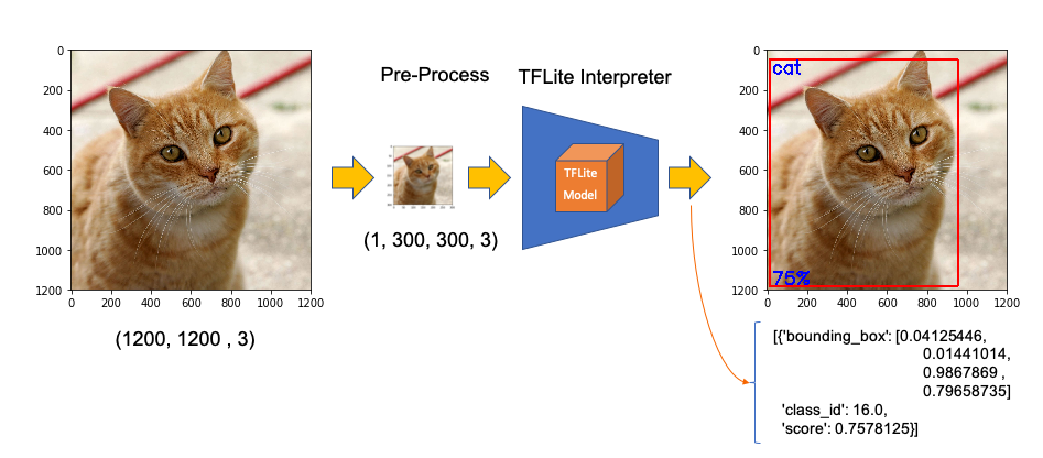
对新图像执行推理的步骤与“图像分类”所执行的步骤非常相似，不同之处在于：

• input: image must have a shape of 300x300 pixels
  输入：图片的形状必须为300x300像素
• output: include not only label and probability (“score”), but also the relative window position (“ Bounding Box”) about where the object is located on the image.
  输出：不仅包括标签和概率(“分数”)，还包括有关对象在图像上的位置的相对窗口位置(“边界框”)。

Now, we must load the labels and model, allocating tensors.

现在，我们必须加载标签和模型，并分配张量。

labels = load_labels('./models/coco_labels.txt')interpreter = Interpreter('./models/detect.tflite')interpreter.allocate_tensors()

The input pre-process is the same as we did before, but the output should be worked to get a more readable output. The functions below will help with that:

输入的预处理与我们之前的相同，但是应该对输出进行处理以获得更易读的输出。 以下功能将帮助您：

def set_input_tensor(interpreter, image):    """Sets the input tensor."""    tensor_index = interpreter.get_input_details()[0]['index']    input_tensor = interpreter.tensor(tensor_index)()[0]    input_tensor[:, :] = imagedef get_output_tensor(interpreter, index):    """Returns the output tensor at the given index."""    output_details = interpreter.get_output_details()[index]    tensor = np.squeeze(interpreter.get_tensor(output_details['index']))    return tensor

With the help of the above functions, detect_objects() will return the inference results:

借助以上功能，detect_objects()将返回推断结果：

• object label id
  对象标签ID
• score
  得分
• the bounding box, that will show where the object is located.
  边界框，它将显示对象的位置。

We have included a ‘threshold’ to avoid objects with a low probability of being correct. Usually, we should consider a score above 50%.

我们包含了一个“阈值”，以避免物体正确的可能性很小。 通常，我们应该考虑分数高于50％。

def detect_objects(interpreter, image, threshold):    set_input_tensor(interpreter, image)    interpreter.invoke()

    # Get all output details    boxes = get_output_tensor(interpreter, 0)    classes = get_output_tensor(interpreter, 1)    scores = get_output_tensor(interpreter, 2)    count = int(get_output_tensor(interpreter, 3))    results = []    for i in range(count):        if scores[i] >= threshold:            result = {                'bounding_box': boxes[i],                'class_id': classes[i],                'score': scores[i]            }            results.append(result)    return results

If we apply the above function to a reshaped image (same as used on classification example), we should get:

如果将上述功能应用于重塑图像(与分类示例相同)，则应获得：

Great! In less than 200ms with 77% probability, an object with id 16 was detected on an area delimited by a ‘bounding box’: (0.028011084, 0.020121813, 0.9886069, 0.802299). Those four numbers are respectively related to ymin, xmin, ymax and xmax.

大！ 在不到200毫秒的时间内以77％的概率在由“边界框”界定的区域上检测到ID为16的对象：(0.028011084、0.020121813、0.9886069、0.802299)。 这四个数字分别与ymin，xmin，ymax和xmax有关。

Take into consideration that y goes from the top (ymin) to bottom (ymax) and x goes from left (xmin) to the right (xmax) as shown in figure below:

考虑到y从顶部(ymin)到底部(ymax)，x从左侧(xmin)到右侧(xmax)，如下图所示：

Having the bounding box four values, we have, in fact, the coordinates of the top/left corner and the bottom/right one. With both edges and knowing the shape of the picture, it is possible to draw the rectangle around the object.

边界框有四个值，实际上，我们有上/左角和下/右角的坐标。 有了两条边缘并知道图片的形状，就可以在对象周围绘制矩形。

Next, we should find what class_id equal to 16 means. Opening the file coco_labels.txt, as a dictionary, each of its elements has an index associated, and inspecting index 16, we get as expected, ‘cat.’ The probability is the value returning from the score.

接下来，我们应该找到等于16的class_id。 打开文件coco_labels.txt作为字典，它的每个元素都有一个关联的索引，并检查索引16，我们得到的是预期的“猫”。 概率是从分数返回的值。

Let’s create a general function to detect multiple objects on a single picture. The first function, starting from an image path, will execute the inference, returning the resized image and the results (multiples ids, each one with its scores and bounding boxes:

让我们创建一个常规功能来检测单个图片上的多个对象。 第一个函数从图像路径开始，将执行推理，返回调整大小的图像和结果(多个id，每个id都有其得分和边界框：

def detectObjImg_2(image_path, threshold = 0.51):img = cv2.imread(image_path)    img = cv2.cvtColor(img, cv2.COLOR_BGR2RGB)    image = cv2.resize(img, (width, height),                       fx=0.5,                       fy=0.5,                       interpolation=cv2.INTER_AREA)    results = detect_objects(interpreter, image, threshold)return img, results

Having the reshaped image, and inference results, the below function can be used to draw a rectangle around the objects, specifying for each one, its label and probability:

具有重塑的图像和推断结果后，以下功能可用于在对象周围绘制一个矩形，并为每个对象指定其标签和概率：

def detect_mult_object_picture(img, results):    HEIGHT, WIDTH, _ = img.shape    aspect = WIDTH / HEIGHT    WIDTH = 640    HEIGHT = int(640 / aspect)    dim = (WIDTH, HEIGHT)   img = cv2.resize(img, dim, interpolation=cv2.INTER_AREA)   for i in range(len(results)):        id = int(results[i]['class_id'])        prob = int(round(results[i]['score'], 2) * 100)

        ymin, xmin, ymax, xmax = results[i]['bounding_box']        xmin = int(xmin * WIDTH)        xmax = int(xmax * WIDTH)        ymin = int(ymin * HEIGHT)        ymax = int(ymax * HEIGHT)        text = "{}: {}%".format(labels[id], prob)        if ymin > 10: ytxt = ymin - 10        else: ytxt = ymin + 15        img = cv2.rectangle(img, (xmin, ymin), (xmax, ymax),                            COLORS[id],                            thickness=2)        img = cv2.putText(img, text, (xmin + 3, ytxt), FONT, 0.5, COLORS[id],                          2)   return img

Below some results:

下面是一些结果：

The complete code can be found at GitHub.

完整的代码可以在GitHub上找到 。

使用相机进行物体检测 (Object Detection using Camera)

If you have a PiCam connected to Raspberry Pi, it is possible to capture a video and perform object recognition, frame by frame, using the same functions defined before. Please follow this tutorial if you do not have a working camera in your Pi: Getting started with the Camera Module.

如果您将PiCam连接到Raspberry Pi，则可以使用之前定义的相同功能来捕获视频并逐帧执行对象识别。 如果您的Pi中没有可使用的相机，请按照本教程进行操作： 相机模块入门 。

First, it is essential to define the size of the frame to be captured by the camera. We will use 640x480.

首先，必须定义相机要拍摄的画面尺寸。 我们将使用640x480。

WIDTH = 640HEIGHT = 480

Next, you must iniciate the camera:

接下来，您必须启动摄像头：

cap = cv2.VideoCapture(0)cap.set(3, WIDTH)cap.set(4, HEIGHT)

And run the below code in a loop. Until the key ‘q’ is pressed, the camera will capture the video, frame by frame, drawing the bounding box with its respective labels and probabilities.

并循环运行以下代码。 在按下键“ q”之前，摄像机将逐帧捕获视频，并绘制带有相应标签和概率的边界框。

while True:    timer = cv2.getTickCount()    success, img = cap.read()    img = cv2.flip(img, 0)    img = cv2.flip(img, 1)    fps = cv2.getTickFrequency() / (cv2.getTickCount() - timer)    cv2.putText(img, "FPS: " + str(int(fps)), (10, 470),                cv2.FONT_HERSHEY_SIMPLEX, 0.7, (0, 0, 255), 2)    image = cv2.cvtColor(img, cv2.COLOR_BGR2RGB)    image = cv2.resize(image, (width, height),                       fx=0.5,                       fy=0.5,                       interpolation=cv2.INTER_AREA)    start_time = time.time()    results = detect_objects(interpreter, image, 0.55)    elapsed_ms = (time.time() - start_time) * 1000    img = detect_mult_object_picture(img, results)    cv2.imshow("Image Recognition ==> Press [q] to Exit", img)if cv2.waitKey(1) & 0xFF == ord('q'):        breakcap.release()cv2.destroyAllWindows()

Below is possible to see the video running in real-time on the Raspberry Pi screen. Note that the video runs around 60 FPS (frames per second), which is pretty good!.

下面可以在Raspberry Pi屏幕上实时观看视频。 请注意，视频的运行速度约为60 FPS(每秒帧数)，非常好！

演示地址

Here one screen-shot of the above video:

以下是上述视频的屏幕截图：

The complete code is available on GitHub.

完整的代码可在GitHub上获得。

姿势估计 (Pose Estimation)

One of the more exciting and critical areas of AI is to estimate a person’s real-time pose, enabling machines to understand what people are doing in images and videos. Pose estimation was deeply explored in my article Realtime Multiple Person 2D Pose Estimation using TensorFlow2.x, but here at the Edge, with a Raspberry Pi and with the help of TensorFlow Lite, it is possible to easily replicate almost the same that was done on a Mac.

AI的一个更令人激动和关键的领域之一是估计一个人的实时姿势，使机器能够了解人们在图像和视频中正在做什么。 在我的文章中使用TensorFlow2.x进行了实时多人2D姿势估计，对姿势估计进行了深入探讨，但是在Edge上，借助Raspberry Pi和TensorFlow Lite的帮助，可以轻松地复制几乎与以前相同的姿势 Mac。

The model that we will use in this project is the PoseNet. We will do inference the same way done for Image Classification and Object Detection, where an image is fed through a pre-trained model. PoseNet comes with a few different versions of the model, corresponding to variances of MobileNet v1 architecture and ResNet50 architecture. In this project, the version pre-trained is the MobileNet V1, which is smaller, faster, but less accurate than ResNet. Also, there are separate models for single and multiple person pose detection. We will explore the model trained for a single person.

我们将在此项目中使用的模型是PoseNet 。 我们将以与图像分类和对象检测相同的方式进行推理，其中图像通过预训练的模型进行馈送。 PoseNet带有一些模型的不同版本，对应于MobileNet v1架构和ResNet50架构的差异。 在此项目中，预培训的版本是MobileNet V1，它比ResNet较小，更快，但准确性较低。 此外，还有用于单人和多人姿势检测的单独模型。 我们将探索为一个人训练的模型。

In this site is possible to explore in real time and using a live camera, several PoseNet models and configurations.

在此站点中，可以使用实时摄像机实时浏览多种PoseNet模型和配置。

The libraries to execute Pose Estimation on a Raspberry Pi are the same used before. NumPy, MatPlotLib, OpenCV and TensorFlow Lite Interpreter.

在Raspberry Pi上执行姿势估计的库与以前使用的库相同。 NumPy，MatPlotLib，OpenCV和TensorFlow Lite解释器。

The pre-trained model is the posenet_mobilenet_v1_100_257x257_multi_kpt_stripped.tflite, which can be downloaded from the above link or the TensorFlow Lite — Pose Estimation Overview website. The model should be saved in the models subdirectory.

预先训练的模型是posenet_mobilenet_v1_100_257x257_multi_kpt_stripped.tflite ，可以从上面的链接或TensorFlow Lite- 姿势估计概述网站下载 。 该模型应保存在models子目录中。

Start loading TFLite model and allocating tensors:

开始加载TFLite模型并分配张量：

interpreter = tflite.Interpreter(model_path='./models/posenet_mobilenet_v1_100_257x257_multi_kpt_stripped.tflite')interpreter.allocate_tensors()

Get input and output tensors:

获取输入和输出张量：

input_details = interpreter.get_input_details()output_details = interpreter.get_output_details()

Same as we did before, looking into the input_details, it is possible to see that the image to be used to pose estimation should be (1, 257, 257, 3), which means that images must be reshaped to 257x257 pixels.

与我们之前所做的一样，查看input_details，可以看到用于姿势估计的图像应为(1，257，257，3)，这意味着必须将图像重塑为257x257像素。

Let’s take as input a simple human figure, that will help us to analyze it:

让我们以一个简单的人物作为输入，这将帮助我们对其进行分析：

The first step is to pre-process the image. This particular model was not quantized, which means that the dtype is float32. This information is essential to pre-process the input image, as shown with the below code

第一步是预处理图像。 此特定模型未量化，这意味着dtype为float32。 此信息对于预处理输入图像至关重要，如以下代码所示

image = cv2.resize(image, size) input_data = np.expand_dims(image, axis=0)input_data = input_data.astype(np.float32)input_data = (np.float32(input_data) - 127.5) / 127.5

Having the image pre-processed, now it is time to perform the inference, feeding the tensor with the image and invoking the interpreter:

对图像进行预处理后，现在该执行推理了，向张量提供图像并调用解释器：

interpreter.set_tensor(input_details[0]['index'], input_data)interpreter.invoke()

An article that helps a lot to understand how to work with PoseNet is the Ivan Kunyakin tutorial’s Pose estimation and matching with TensorFlow lite. There Ivan comments that on the output vector, what matters to find the key points, are:

Ivan Kunyakin教程的Pose估计以及与TensorFlow lite的匹配，对帮助您理解如何使用PoseNet 很有帮助 。 Ivan评论说，在输出向量上，找到关键点很重要：

• Heatmaps 3D tensor of size (9,9,17), that corresponds to the probability of appearance of each one of the 17 keypoints (body joints) in the particular part of the image (9,9). It is used to locate the approximate position of the joint.

  热图大小为(9,9,17)的3D张量，它对应于图像的特定部分(9,9)中17个关键点(身体关节)中的每一个出现的概率。 用于定位关节的大致位置。

• Offset Vectors: 3D tensor of size (9,9,34) that is called offset vectors. It is used for more exact calculation of the keypoint’s position. The First 17 of the third dimension correspond to the x coordinates and the second 17 of them to the y coordinates.

  偏移向量：大小为(9,9,34)的3D张量，称为偏移向量。 它用于更精确地计算关键点的位置。 三维的第一个17对应于x坐标，第二个17对应于y坐标。

output_details = interpreter.get_output_details()[0]heatmaps = np.squeeze(interpreter.get_tensor(output_details['index']))output_details = interpreter.get_output_details()[1]offsets = np.squeeze(interpreter.get_tensor(output_details['index']))

Let’s create a function that will return an array with all 17 keypoints (or person's joints) based on heatmaps and offsets.

让我们创建一个函数，该函数将根据热图和偏移量返回一个包含所有17个关键点(或人的关节)的数组。

def get_keypoints(heatmaps, offsets):    joint_num = heatmaps.shape[-1]    pose_kps = np.zeros((joint_num, 2), np.uint32)    max_prob = np.zeros((joint_num, 1))    for i in range(joint_num):        joint_heatmap = heatmaps[:,:,i]        max_val_pos = np.squeeze(            np.argwhere(joint_heatmap == np.max(joint_heatmap)))        remap_pos = np.array(max_val_pos / 8 * 257, dtype=np.int32)        pose_kps[i, 0] = int(remap_pos[0] +                             offsets[max_val_pos[0], max_val_pos[1], i])        pose_kps[i, 1] = int(remap_pos[1] +                             offsets[max_val_pos[0], max_val_pos[1],                                         i + joint_num])        max_prob[i] = np.amax(joint_heatmap)    return pose_kps, max_prob

Using the above function with the heatmaps and offset vectors that were extracted from the output tensor, resultant of the image inference, we get:

使用上面的函数和从输出张量提取的热图和偏移矢量，即图像推断的结果，我们得到：

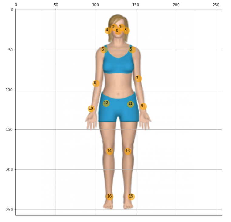
The resultant array shows all 17 coordinates (y, x) regarding where the joints are located on an image of 257 x 257 pixels. Using the code below. It is possible to plot each one of the joints over the resized image. For reference, the array index is annotated, so it is easy to identify each joint:

所得数组显示有关关节在257 x 257像素的图像上的位置的所有17个坐标(y，x)。 使用下面的代码。 可以在调整大小后的图像上绘制每个关节。 作为参考，对数组索引进行了注释，因此很容易识别每个关节：

y,x = zip(*keypts_array)plt.figure(figsize=(10,10))plt.axis([0, image.shape[1], 0, image.shape[0]])  plt.scatter(x,y, s=300, color='orange', alpha=0.6)img = cv2.cvtColor(image, cv2.COLOR_BGR2RGB)plt.imshow(img)ax=plt.gca() ax.set_ylim(ax.get_ylim()[::-1]) ax.xaxis.tick_top() plt.grid();for i, txt in enumerate(keypts_array):    ax.annotate(i, (keypts_array[i][1]-3, keypts_array[i][0]+1))

As a result, we get the picure:

结果，我们得到如下图：

Great, now it is time to create a general function to draw “the bones”, which is the joints’ connection. The bones will be drawn as lines, which are the connections among keypoints 5 to 16, as shown in the above figure. Independent circles will be used for keypoints 0 to 4, related to head:

太好了，现在是时候创建绘制“骨骼”的通用功能了，这是关节的连接。 骨骼将绘制为线，即关键点5到16之间的连接，如上图所示。 独立的圆圈将用于与头部相关的关键点0到4：

def join_point(img, kps, color='white', bone_size=1):

    if   color == 'blue'  : color=(255, 0, 0)    elif color == 'green': color=(0, 255, 0)    elif color == 'red':  color=(0, 0, 255)    elif color == 'white': color=(255, 255, 255)    else:                  color=(0, 0, 0)    body_parts = [(5, 6), (5, 7), (6, 8), (7, 9), (8, 10), (11, 12), (5, 11),                  (6, 12), (11, 13), (12, 14), (13, 15), (14, 16)]    for part in body_parts:        cv2.line(img, (kps[part[0]][1], kps[part[0]][0]),                (kps[part[1]][1], kps[part[1]][0]),                color=color,                lineType=cv2.LINE_AA,                thickness=bone_size)

    for i in range(0,len(kps)):        cv2.circle(img,(kps[i,1],kps[i,0]),2,(255,0,0),-1)

Calling the function, we have the estimated pose of the body in the image:

调用该函数，我们可以在图像中获得人体的估计姿势：

join_point(img, keypts_array, bone_size=2)plt.figure(figsize=(10,10))plt.imshow(img);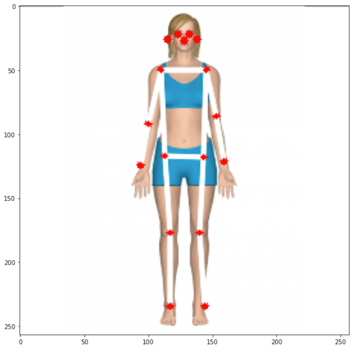

And last but not least, let’s create a general function to estimate posture having an image path as a start:

最后但并非最不重要的一点，我们创建一个通用函数来估计以图像路径作为起点的姿势：

def plot_pose(img, keypts_array, joint_color='red', bone_color='blue', bone_size=1):    join_point(img, keypts_array, bone_color, bone_size)    y,x = zip(*keypts_array)    plt.figure(figsize=(10,10))    plt.axis([0, img.shape[1], 0, img.shape[0]])      plt.scatter(x,y, s=100, color=joint_color)    img = cv2.cvtColor(img, cv2.COLOR_BGR2RGB)    plt.imshow(img)    ax=plt.gca()     ax.set_ylim(ax.get_ylim()[::-1])     ax.xaxis.tick_top()     plt.grid();    return imgdef get_plot_pose(image_path, size, joint_color='red', bone_color='blue', bone_size=1):        image_original = cv2.imread(image_path)    image = cv2.resize(image_original, size)     input_data = np.expand_dims(image, axis=0)    input_data = input_data.astype(np.float32)    input_data = (np.float32(input_data) - 127.5) / 127.5    interpreter.set_tensor(input_details[0]['index'], input_data)    interpreter.invoke()

    output_details = interpreter.get_output_details()[0]    heatmaps = np.squeeze(interpreter.get_tensor(output_details['index']))    output_details = interpreter.get_output_details()[1]    offsets = np.squeeze(interpreter.get_tensor(output_details['index']))    keypts_array, max_prob = get_keypoints(heatmaps,offsets)    orig_kps = get_original_pose_keypoints(image_original, keypts_array, size)    img = plot_pose(image_original, orig_kps, joint_color, bone_color, bone_size)

    return orig_kps, max_prob, img

At this point with only one line of code, it is possible to detect pose on images:

此时，仅需一行代码，就可以检测图像上的姿势：

keypts_array, max_prob, img  = get_plot_pose(image_path, size, bone_size=3)

All code developed on this section is available on GitHub.

在本节中开发的所有代码都可以在GitHub上找到 。

Another easy step is to apply the function to frames from videos and live camera. I will leave it for you! ;-)

另一个简单的步骤是将功能应用于视频和实时摄像机的帧。 我会留给你的！ ;-)

结论 (Conclusion)

TensorFlow Lite is a great framework to implement Artificial Intelligence (more precisely, ML) at the Edge. Here we explored ML models working on a Raspberry Pi, but TFLite is now more and more used at the "edge of the edge", on very small microcontrollers, in what has been called TinyML.

TensorFlow Lite是在Edge上实施人工智能(更准确地说是ML)的绝佳框架。 在这里，我们探索了在Raspberry Pi上运行的ML模型，但是现在TFLite越来越多地在称为TinyML的非常小的微控制器上的“边缘边缘” 使用 。

As always, I hope this article can inspire others to find their way in the fantastic world of AI!

与往常一样，我希望本文能够激发其他人在梦幻般的AI世界中找到自己的路！

All the codes used in this article are available for download on project GitHub: TFLite_IA_at_the_Edge.

本文中使用的所有代码都可以在GitHub项目TFLite_IA_at_the_Edge上下载。

Regards from the South of the World!

南方的问候！

See you in my next article!

下一篇再见！

Thank you

谢谢

Marcelo

马塞洛