Machine Learning from Start to Finish with Scikit-Learn
2019独角兽企业重金招聘Python工程师标准>>> 
Machine Learning from Start to Finish with Scikit-Learn
This notebook covers the basic Machine Learning process in Python step-by-step. Go from raw data to at least 78% accuracy on the Titanic Survivors dataset.
Steps Covered
- Importing a DataFrame
- Visualize the Data
- Cleanup and Transform the Data
- Encode the Data
- Split Training and Test Sets
- Fine Tune Algorithms
- Cross Validate with KFold
- Upload to Kaggle
CSV to DataFrame
CSV files can be loaded into a dataframe by calling pd.read_csv . After loading the training and test files, print a sample to see what you're working with.
In [1]:
import numpy as np
import pandas as pd
import matplotlib.pyplot as plt
import seaborn as sns
%matplotlib inlinedata_train = pd.read_csv('../input/train.csv')
data_test = pd.read_csv('../input/test.csv')data_train.sample(3)
Out[1]:
| PassengerId | Survived | Pclass | Name | Sex | Age | SibSp | Parch | Ticket | Fare | Cabin | Embarked | |
|---|---|---|---|---|---|---|---|---|---|---|---|---|
| 47 | 48 | 1 | 3 | O'Driscoll, Miss. Bridget | female | NaN | 0 | 0 | 14311 | 7.7500 | NaN | Q |
| 296 | 297 | 0 | 3 | Hanna, Mr. Mansour | male | 23.5 | 0 | 0 | 2693 | 7.2292 | NaN | C |
| 530 | 531 | 1 | 2 | Quick, Miss. Phyllis May | female | 2.0 | 1 | 1 | 26360 | 26.0000 | NaN | S |
Visualizing Data
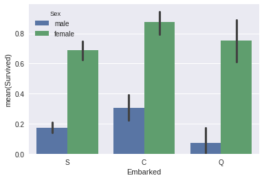
Visualizing data is crucial for recognizing underlying patterns to exploit in the model.
In [2]:
sns.barplot(x="Embarked", y="Survived", hue="Sex", data=data_train);
In [3]:
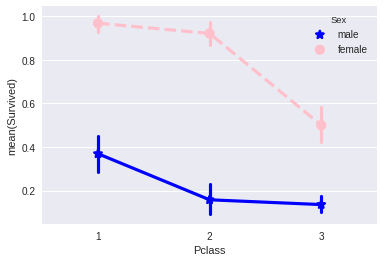
sns.pointplot(x="Pclass", y="Survived", hue="Sex", data=data_train,palette={"male": "blue", "female": "pink"},markers=["*", "o"], linestyles=["-", "--"]);
Transforming Features
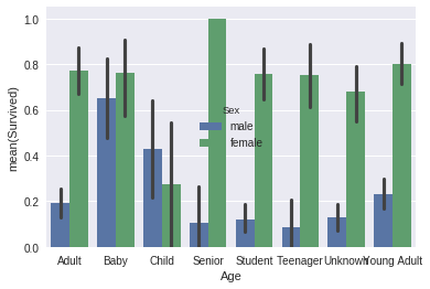
- Aside from 'Sex', the 'Age' feature is second in importance. To avoid overfitting, I'm grouping people into logical human age groups.
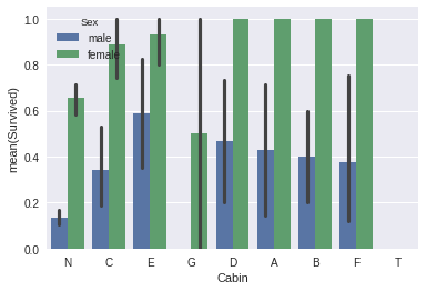
- Each Cabin starts with a letter. I bet this letter is much more important than the number that follows, let's slice it off.
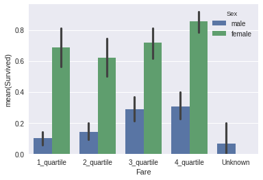
- Fare is another continuous value that should be simplified. I ran
data_train.Fare.describe()to get the distribution of the feature, then placed them into quartile bins accordingly. - Extract information from the 'Name' feature. Rather than use the full name, I extracted the last name and name prefix (Mr. Mrs. Etc.), then appended them as their own features.
- Lastly, drop useless features. (Ticket and Name)
In [4]:
def simplify_ages(df):df.Age = df.Age.fillna(-0.5)bins = (-1, 0, 5, 12, 18, 25, 35, 60, 120)group_names = ['Unknown', 'Baby', 'Child', 'Teenager', 'Student', 'Young Adult', 'Adult', 'Senior']categories = pd.cut(df.Age, bins, labels=group_names)df.Age = categoriesreturn dfdef simplify_cabins(df):df.Cabin = df.Cabin.fillna('N')df.Cabin = df.Cabin.apply(lambda x: x[0])return dfdef simplify_fares(df):df.Fare = df.Fare.fillna(-0.5)bins = (-1, 0, 8, 15, 31, 1000)group_names = ['Unknown', '1_quartile', '2_quartile', '3_quartile', '4_quartile']categories = pd.cut(df.Fare, bins, labels=group_names)df.Fare = categoriesreturn dfdef format_name(df):df['Lname'] = df.Name.apply(lambda x: x.split(' ')[0])df['NamePrefix'] = df.Name.apply(lambda x: x.split(' ')[1])return df    def drop_features(df):return df.drop(['Ticket', 'Name', 'Embarked'], axis=1)def transform_features(df):df = simplify_ages(df)df = simplify_cabins(df)df = simplify_fares(df)df = format_name(df)df = drop_features(df)return dfdata_train = transform_features(data_train)
data_test = transform_features(data_test)
data_train.head()
Out[4]:
| PassengerId | Survived | Pclass | Sex | Age | SibSp | Parch | Fare | Cabin | Lname | NamePrefix | |
|---|---|---|---|---|---|---|---|---|---|---|---|
| 0 | 1 | 0 | 3 | male | Student | 1 | 0 | 1_quartile | N | Braund, | Mr. |
| 1 | 2 | 1 | 1 | female | Adult | 1 | 0 | 4_quartile | C | Cumings, | Mrs. |
| 2 | 3 | 1 | 3 | female | Young Adult | 0 | 0 | 1_quartile | N | Heikkinen, | Miss. |
| 3 | 4 | 1 | 1 | female | Young Adult | 1 | 0 | 4_quartile | C | Futrelle, | Mrs. |
| 4 | 5 | 0 | 3 | male | Young Adult | 0 | 0 | 2_quartile | N | Allen, | Mr. |
In [5]:
In [5]:
sns.barplot(x="Age", y="Survived", hue="Sex", data=data_train);
In [6]:
sns.barplot(x="Cabin", y="Survived", hue="Sex", data=data_train);
In [7]:
sns.barplot(x="Fare", y="Survived", hue="Sex", data=data_train);
Some Final Encoding
The last part of the preprocessing phase is to normalize labels. The LabelEncoder in Scikit-learn will convert each unique string value into a number, making out data more flexible for various algorithms.
The result is a table of numbers that looks scary to humans, but beautiful to machines.
In [8]:
from sklearn import preprocessing
def encode_features(df_train, df_test):features = ['Fare', 'Cabin', 'Age', 'Sex', 'Lname', 'NamePrefix']df_combined = pd.concat([df_train[features], df_test[features]])for feature in features:le = preprocessing.LabelEncoder()le = le.fit(df_combined[feature])df_train[feature] = le.transform(df_train[feature])df_test[feature] = le.transform(df_test[feature])return df_train, df_testdata_train, data_test = encode_features(data_train, data_test)
data_train.head()
Out[8]:
| PassengerId | Survived | Pclass | Sex | Age | SibSp | Parch | Fare | Cabin | Lname | NamePrefix | |
|---|---|---|---|---|---|---|---|---|---|---|---|
| 0 | 1 | 0 | 3 | 1 | 4 | 1 | 0 | 0 | 7 | 100 | 19 |
| 1 | 2 | 1 | 1 | 0 | 0 | 1 | 0 | 3 | 2 | 182 | 20 |
| 2 | 3 | 1 | 3 | 0 | 7 | 0 | 0 | 0 | 7 | 329 | 16 |
| 3 | 4 | 1 | 1 | 0 | 7 | 1 | 0 | 3 | 2 | 267 | 20 |
| 4 | 5 | 0 | 3 | 1 | 7 | 0 | 0 | 1 | 7 | 15 | 19 |
Splitting up the Training Data
Now its time for some Machine Learning.
First, separate the features(X) from the labels(y).
X_all: All features minus the value we want to predict (Survived).
y_all: Only the value we want to predict.
Second, use Scikit-learn to randomly shuffle this data into four variables. In this case, I'm training 80% of the data, then testing against the other 20%.
Later, this data will be reorganized into a KFold pattern to validate the effectiveness of a trained algorithm.
In [9]:
from sklearn.model_selection import train_test_splitX_all = data_train.drop(['Survived', 'PassengerId'], axis=1)
y_all = data_train['Survived']num_test = 0.20
X_train, X_test, y_train, y_test = train_test_split(X_all, y_all, test_size=num_test, random_state=23)
Fitting and Tuning an Algorithm
Now it's time to figure out which algorithm is going to deliver the best model. I'm going with the RandomForestClassifier, but you can drop any other classifier here, such as Support Vector Machines or Naive Bayes.
In [10]:
from sklearn.ensemble import RandomForestClassifier
from sklearn.metrics import make_scorer, accuracy_score
from sklearn.model_selection import GridSearchCV# Choose the type of classifier.
clf = RandomForestClassifier()# Choose some parameter combinations to try
parameters = {'n_estimators': [4, 6, 9], 'max_features': ['log2', 'sqrt','auto'], 'criterion': ['entropy', 'gini'],'max_depth': [2, 3, 5, 10], 'min_samples_split': [2, 3, 5],'min_samples_leaf': [1,5,8]}# Type of scoring used to compare parameter combinations
acc_scorer = make_scorer(accuracy_score)# Run the grid search
grid_obj = GridSearchCV(clf, parameters, scoring=acc_scorer)
grid_obj = grid_obj.fit(X_train, y_train)# Set the clf to the best combination of parameters
clf = grid_obj.best_estimator_# Fit the best algorithm to the data.
clf.fit(X_train, y_train)
Out[10]:
RandomForestClassifier(bootstrap=True, class_weight=None, criterion='entropy',max_depth=5, max_features='sqrt', max_leaf_nodes=None,min_impurity_decrease=0.0, min_impurity_split=None,min_samples_leaf=1, min_samples_split=3,min_weight_fraction_leaf=0.0, n_estimators=9, n_jobs=1,oob_score=False, random_state=None, verbose=0,warm_start=False)
In [11]:
predictions = clf.predict(X_test)
print(accuracy_score(y_test, predictions))
0.798882681564
Validate with KFold
Is this model actually any good? It helps to verify the effectiveness of the algorithm using KFold. This will split our data into 10 buckets, then run the algorithm using a different bucket as the test set for each iteration.
In [12]:
from sklearn.cross_validation import KFolddef run_kfold(clf):kf = KFold(891, n_folds=10)outcomes = []fold = 0for train_index, test_index in kf:fold += 1X_train, X_test = X_all.values[train_index], X_all.values[test_index]y_train, y_test = y_all.values[train_index], y_all.values[test_index]clf.fit(X_train, y_train)predictions = clf.predict(X_test)accuracy = accuracy_score(y_test, predictions)outcomes.append(accuracy)print("Fold {0} accuracy: {1}".format(fold, accuracy)) mean_outcome = np.mean(outcomes)print("Mean Accuracy: {0}".format(mean_outcome)) run_kfold(clf)
Fold 1 accuracy: 0.8111111111111111
Fold 2 accuracy: 0.8651685393258427
Fold 3 accuracy: 0.7640449438202247
Fold 4 accuracy: 0.8426966292134831
Fold 5 accuracy: 0.8314606741573034
Fold 6 accuracy: 0.8202247191011236
Fold 7 accuracy: 0.7528089887640449
Fold 8 accuracy: 0.8089887640449438
Fold 9 accuracy: 0.8876404494382022
Fold 10 accuracy: 0.8426966292134831
Mean Accuracy: 0.8226841448189763
/opt/conda/lib/python3.6/site-packages/sklearn/cross_validation.py:41: DeprecationWarning: This module was deprecated in version 0.18 in favor of the model_selection module into which all the refactored classes and functions are moved. Also note that the interface of the new CV iterators are different from that of this module. This module will be removed in 0.20."This module will be removed in 0.20.", DeprecationWarning)
Predict the Actual Test Data
And now for the moment of truth. Make the predictions, export the CSV file, and upload them to Kaggle.
In [13]:
ids = data_test['PassengerId']
predictions = clf.predict(data_test.drop('PassengerId', axis=1))output = pd.DataFrame({ 'PassengerId' : ids, 'Survived': predictions })
# output.to_csv('titanic-predictions.csv', index = False)
output.head()
Out[13]:
| PassengerId | Survived | |
|---|---|---|
| 0 | 892 | 0 |
| 1 | 893 | 0 |
| 2 | 894 | 0 |
| 3 | 895 | 0 |
| 4 | 896 | 0 |
转载于:https://my.oschina.net/cloudcoder/blog/1068712
Machine Learning from Start to Finish with Scikit-Learn相关推荐
- 《Hands-On Machine Learning with Scikit-Learn TensorFlow》读书笔记(一):机器学习概述
最近有时间看书了,把以前想看的书捡一下,翻译中顺便加上自己的理解,写个读书笔记. 一.什么是机器学习? Machine Learning is the science (and art) of pro ...
- bff v2ex_语音备忘录的BFF-如何通过Machine Learning简化Speech2Text
bff v2ex by Rafael Belchior 通过拉斐尔·贝尔基奥尔(Rafael Belchior) 语音备忘录的BFF-如何通过Machine Learning简化Speech2Text ...
- Machine Learning | (2) sklearn数据集与机器学习组成
Machine Learning | 机器学习简介 Machine Learning | (1) Scikit-learn与特征工程 Machine Learning | (2) sklearn数据集 ...
- Python Tools for Machine Learning
2019独角兽企业重金招聘Python工程师标准>>> 原文:https://www.cbinsights.com/blog/python-tools-machine-learnin ...
- 如何在时间紧迫情况下进行机器学习:构建标记的新闻 数据 库 开发 标记 网站 阅读1629 原文:How we built Tagger News: machine learning on a
如何在时间紧迫情况下进行机器学习:构建标记的新闻 数据 库 开发 标记 网站 阅读1629 原文:How we built Tagger News: machine learning on a ti ...
- 机器学习面试题合集Collection of Machine Learning Interview Questions
The Machine Learning part of the interview is usually the most elaborate one. That's the reason we h ...
- AI:《Why is DevOps for Machine Learning so Different?—为什么机器学习的 DevOps 如此不同?》翻译与解读
AI:<Why is DevOps for Machine Learning so Different?-为什么机器学习的 DevOps 如此不同?>翻译与解读 目录 <Why is ...
- Build a Machine Learning Portfolio(构建机器学习投资组合)
Complete Small Focused Projects and Demonstrate Your Skills (完成小型针对性机器学习项目,证明你的能力) A portfolio is ty ...
- machine learning for hacker记录(3) 贝叶斯分类器
本章主要介绍了分类算法里面的一种最基本的分类器:朴素贝叶斯算法(NB),算法性能正如英文缩写的一样,很NB,尤其在垃圾邮件检测领域,关于贝叶斯的网上资料也很多,这里推荐那篇刘未鹏写的http://mi ...
最新文章
- 上海Uber优步司机奖励政策(1月18日~1月24日)
- RxJava学习资源整合
- .net程序员的盲点(一):参数修饰符ref,out ,params的区别
- C# 多线程之List的线程安全问题
- mysql 更新表格数据_mysql更新表格数据库数据
- 算法 --- 递归生成括号
- 国内linux内核镜像仓库,国内较快的maven仓库镜像
- 【Linux】kali linux 安装 google chrome
- 蓝色起源成功完成“新谢泼德号”飞船第17次发射
- 常用的分隔符有哪三种_掌握这三种调漂方法,你想怎么钓就怎么钓,再也不用求人...
- 人工鱼群算法Matlab实现
- 如何使用计算机检测网络正常使用,如何测试网速? 本地测网速的几种方法分享...
- uni-app项目实战
- sqlserver 附加数据库失败,操作系统错误 5:5(拒绝访问。)的解决办法
- 即将创业的我转发一篇鸡汤文---采访了 10 位身价过亿的 CEO,我终于看懂了有钱人的“奋斗”
- 年度征文 | 回顾2022,展望2023(我难忘的2022,我憧憬的2023)
- cocos 安卓打包相关
- 快鲸科技邀您一起合作,共同发展
- clion三角形运行键是灰的_能打游戏能编程,如何用吃灰机器,安装完整ChromeOS(支持安卓)...
- CS61A Lab 13