与AI交易 (Trading with AI)

Stock markets tend to react very quickly to a variety of factors such as news, earnings reports, etc. While it may be prudent to develop trading strategies based on fundamental data, the rapid changes in the stock market are incredibly hard to predict and may not conform to the goals of more short term traders. This study aims to use data science as a means to both identify high potential stocks, as well as attempt to forecast future prices/price movement in an attempt to maximize an investor’s chances of success.

股票市场往往会对各种因素(例如新闻，收益报告等)​​做出快速React。尽管基于基本数据制定交易策略可能是谨慎的做法，但股票市场的快速变化却难以预测，而且可能无法预测符合更多短期交易者的目标。 这项研究旨在利用数据科学来识别高潜力股票，并试图预测未来价格/价格走势，以最大程度地提高投资者的成功机会。

In the first half of this analysis, I will introduce a strategy to search for stocks that involves identifying the highest-ranked stocks based on trading volume during the trading day. I will also include information based on twitter and sentiment analysis in order to provide an idea of which stocks have the maximum probability of going up in the near future. The next half of the project will attempt to apply forecasting techniques to our chosen stock(s). I will apply deep learning via a Long short term memory (LSTM) neural network, which is a form of a recurrent neural network (RNN) to predict close prices. Finally, I will also demonstrate how simple linear regression could aid in forecasting.

在本分析的前半部分，我将介绍一种搜索股票的策略，该策略涉及根据交易日内的交易量来确定排名最高的股票。 我还将包括基于推特和情绪分析的信息，以提供有关哪些股票在不久的将来具有最大上涨可能性的想法。 该项目的下半部分将尝试将预测技术应用于我们选择的股票。 我将通过长期短期记忆(LSTM)神经网络应用深度学习，这是递归神经网络(RNN)的一种形式，可以预测收盘价。 最后，我还将演示简单的线性回归如何有助于预测。

第1部分：库存筛选 (Part 1: Stock screening)

Let’s begin by web-scraping data on the most active stocks in a given time period, in this case, one day. Higher trading volume is more likely to result in bigger price volatility which could potentially result in larger gains. The main python packages to help us with this task are the yahoo_fin, alpha_vantage, and pandas libraries.

首先，在给定的时间段(本例中为一天)中，通过网络收集最活跃的股票的数据。 更高的交易量更有可能导致更大的价格波动，从而有可能带来更大的收益。 可以帮助我们完成此任务的主要python软件包是yahoo_fin ， alpha_vantage和pandas库。

# Import relevant packagesimport yahoo_fin.stock_info as yafrom alpha_vantage.timeseries import TimeSeriesfrom alpha_vantage.techindicators import TechIndicatorsfrom alpha_vantage.sectorperformance import SectorPerformancesimport pandas as pdimport pandas_datareader as webimport matplotlib.pyplot as pltfrom bs4 import BeautifulSoupimport requests import numpy as np# Get the 100 most traded stocks for the trading daymovers = ya.get_day_most_active()movers.head()

The yahoo_fin package is able to provide the top 100 stocks with the largest trading volume. We are interested in stocks with a positive change in price so let’s filter based on that.

yahoo_fin软件包 能够提供交易量最大的前100只股票。 我们对价格有正变化的股票感兴趣，因此让我们基于此进行过滤。

movers = movers[movers['% Change'] >= 0]movers.head()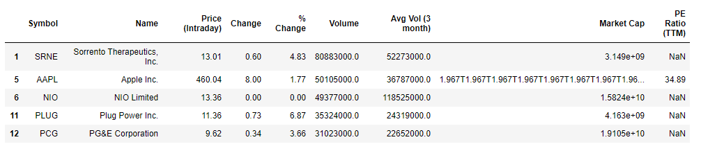

Excellent! We have successfully scraped the data using the yahoo_fin python module. it is often a good idea to see if those stocks are also generating attention, and what kind of attention it is to avoid getting into false rallies. We will scrap some sentiment data courtesy of sentdex. Sometimes sentiments may lag due to source e.g News article published an hour after the event, so we will also utilize tradefollowers for their twitter sentiment data. We will process both lists independently and combine them. For both the sentdex and tradefollowers data we use a 30 day time period. Using a single day might be great for day trading but increases the probability of jumping on false rallies. NOTE: Sentdex only has stocks that belong to the S&P 500. Using the BeautifulSoup library, this process is made fairly simple.

优秀的！ 我们已经使用yahoo_fin python模块成功地抓取了数据。 通常，最好查看这些股票是否也引起关注，以及避免引起虚假集会的关注是什么。 我们将根据senddex删除一些情感数据。 有时，情绪可能会由于消息来源而有所滞后，例如在事件发生后一小时发布的新闻文章，因此我们还将利用贸易关注者的推特情绪数据。 我们将独立处理两个列表并将其合并。 对于senddex和tradefollowers数据，我们使用30天的时间段。 使用单日交易对日间交易而言可能很棒，但会增加跳空虚假反弹的可能性。 注意：Sentdex仅拥有属于S＆P 500的股票。使用BeautifulSoup库，此过程变得相当简单。

res = requests.get('http://www.sentdex.com/financial-analysis/?tf=30d')soup = BeautifulSoup(res.text)table = soup.find_all('tr')# Initialize empty lists to store stock symbol, sentiment and mentionsstock = []sentiment = []mentions = []sentiment_trend = []# Use try and except blocks to mitigate missing datafor ticker in table:    ticker_info = ticker.find_all('td')

    try:        stock.append(ticker_info[0].get_text())    except:        stock.append(None)    try:        sentiment.append(ticker_info[3].get_text())    except:        sentiment.append(None)    try:        mentions.append(ticker_info[2].get_text())    except:        mentions.append(None)    try:        if (ticker_info[4].find('span',{"class":"glyphicon  glyphicon-chevron-up"})):            sentiment_trend.append('up')        else:            sentiment_trend.append('down')    except:        sentiment_trend.append(None)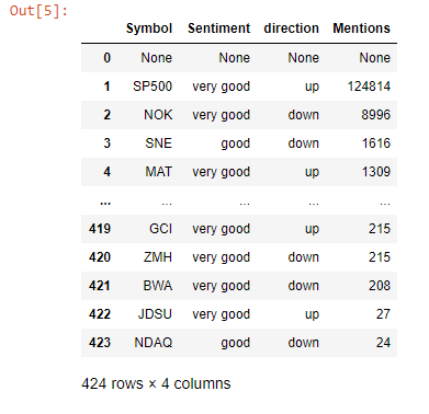

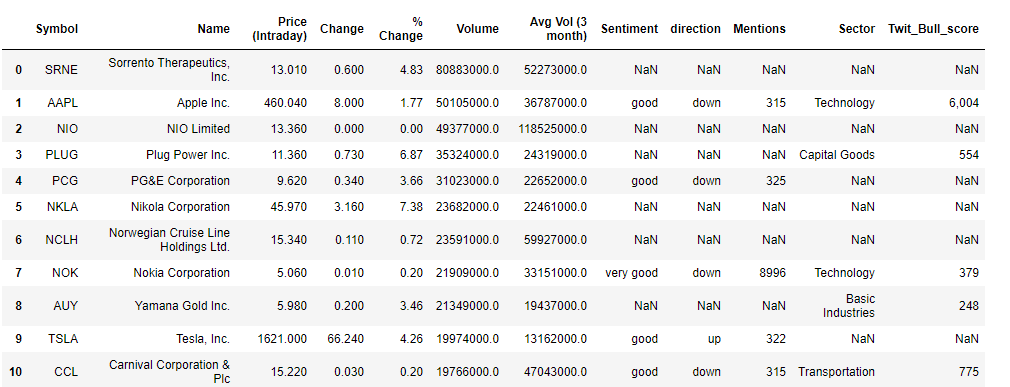
We then combine these results with our previous results about the most traded stocks with positive price changes on a given day. This done using a left join of this data frame with the original movers data frame

然后，我们将这些结果与我们先前的有关交易最多的股票的先前结果相结合，并得出给定价格的正变化。 使用此数据框与原始移动者数据框的左连接完成此操作

top_stocks = movers.merge(company_info, on='Symbol', how='left')top_stocks.drop(['Market Cap','PE Ratio (TTM)'], axis=1, inplace=True)top_stocks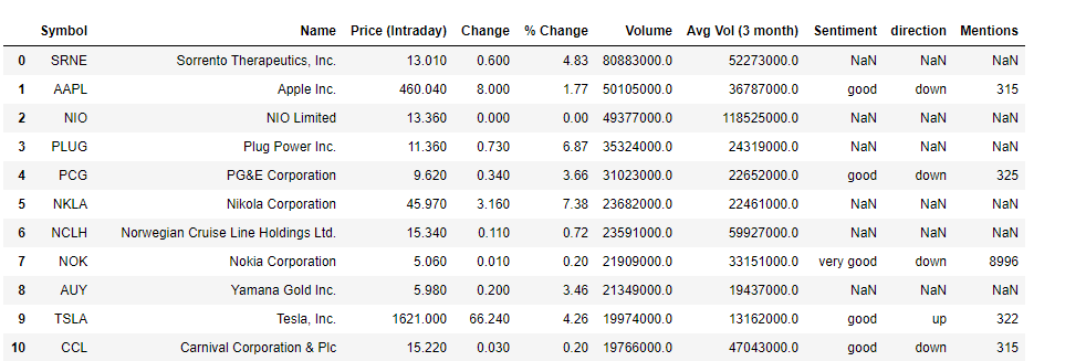

The movers data frame had a total of 45 stocks but for brevity only 10 are shown here. A couple of stocks pop up with both very good sentiments and an upwards trend in favourability. ZNGA, TWTR, and AES (not shown) for instance stood out as potentially good picks. Note, the mentions here refer to the number of times the stock was referenced according to the internal metrics used by sentdex. Let’s attempt supplementing this information with some data based on twitter. We get stocks that showed the strongest twitter sentiments within a time period of 1 month and were considered bullish.

推动者数据框中共有45种存量，但为简洁起见，此处仅显示10种。 情绪高涨且有利可图的趋势呈上升趋势的几只股票。 例如，ZNGA，TWTR和AES(未显示)脱颖而出，成为潜在的好选择。 请注意，此处提及的内容是指根据senddex使用的内部指标引用股票的次数 。 让我们尝试使用基于Twitter的一些数据来补充此信息。 我们得到的股票在1个月内显示出最强烈的Twitter情绪，并被视为看涨。

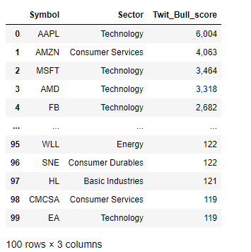
Twit_Bull_score refers to the internal scoring used at tradefollowers to rank stocks that are considered bullish, based on twitter sentiments, and can range from 1 to as high as 10,000 or greater. With the twitter sentiments obtained, I’ll combine it with our sentiment data to get an overall idea of the stocks and their sentiments

Twit_Bull_score指的是在所使用的内部计分tradefollowers到秩股被认为看涨，基于在twitter情绪，并且范围可以从1至高达10,000或更大。 在获得推特情绪后，我将其与情绪数据结合起来以全面了解股票及其情绪

For completeness, stocks classified as having large momentum and their sentiment data will also be included in this analysis. These were scraped and merged with the Final_list data frame.

为了完整起见，被归类为动量较大的股票及其情绪数据也将包括在此分析中。 这些内容已被抓取并与Final_list数据框合并。

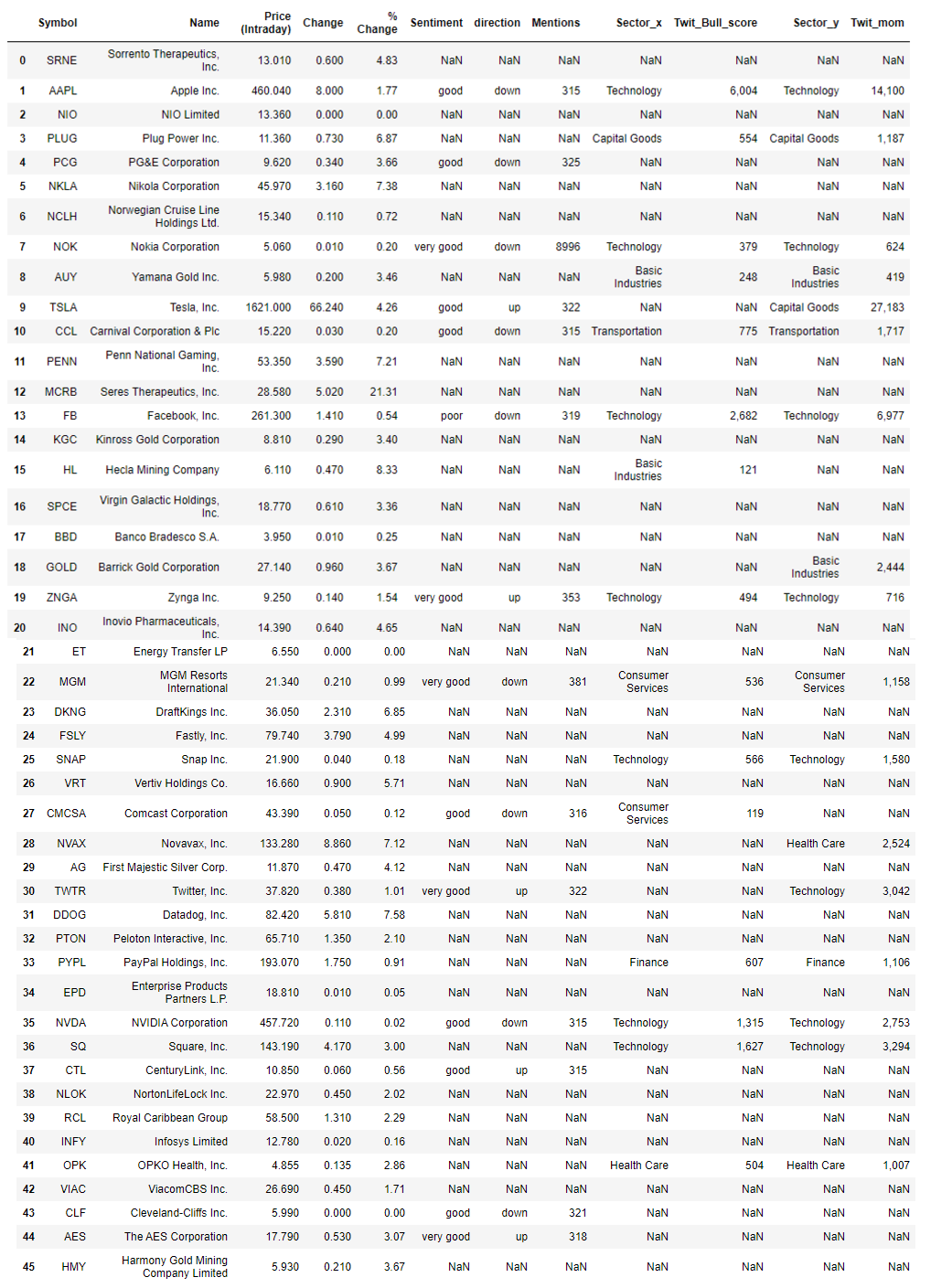
Our list now contains even more information to help us with our trades. Stocks that it suggests might generate positive returns include TSLA, ZNGA, and TWTR as their sentiments are positive, and they have relatively decent twitter sentiment scores. As an added measure, we can also obtain information on the sectors to see how they’ve performed. Again, we will use a one month time period for comparison. The aforementioned stocks belong to the Technology and consumer staples sectors.

我们的清单现在包含更多信息，以帮助我们进行交易。 它暗示可能产生正回报的股票包括TSLA，ZNGA和TWTR，因为它们的情绪是积极的，并且它们的Twitter情绪得分相对不错。 作为一项附加措施，我们还可以获得有关部门的信息，以了解其表现。 同样，我们将使用一个月的时间进行比较。 上述股票属于技术和消费必需品领域。

# Checking sector performancessp = SectorPerformances(key='0E66O7ZP6W7A1LC9', output_format='pandas')plt.figure(figsize=(8,8))data, meta_data = sp.get_sector()print(meta_data)data['Rank D: Month Performance'].plot(kind='bar')plt.title('One Month Performance (%) per Sector')plt.tight_layout()plt.grid()plt.show()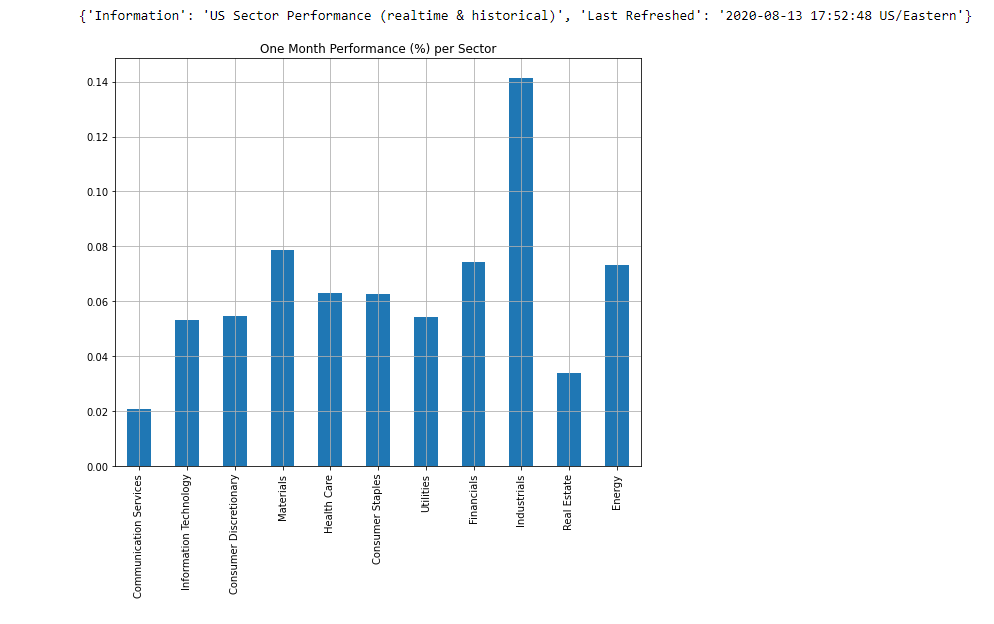

The industrials sector appears to be the best performing in this time period. Consumer staples sector appears to be doing better than the information technology sector, but overall they are up which bodes well for potential investors. Of course with stocks, a combination of news, technical and fundamental analysis, as well as knowledge of the given product/sector, is needed to effectively invest but this system is designed to find stocks that are more likely to perform.

在这段时间内，工业部门表现最好。 消费必需品领域似乎比信息技术领域做得更好，但总体而言，它们的增长对潜在的投资者来说是个好兆头。 当然，对于库存而言，需要新闻，技术和基本面分析以及对给定产品/行业的知识的组合才能有效地进行投资，但是此系统旨在查找更有可能执行的库存。

To validate this notion, let’s construct a mock portfolio using TSLA, ZNGA, and TWTR as our chosen stocks and observe their cumulative returns. This particular analysis began on the 13th of August, 2020 so that will be the starting date of the investments.

为了验证这一观点，让我们使用TSLA，ZNGA和TWTR作为我们选择的股票来构建模拟投资组合，并观察它们的累积收益。 这项特殊的分析始于2020年8月13日，因此这将是投资的开始日期。

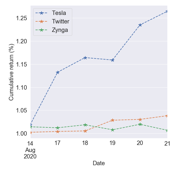
Overall all three investments would have netted a positive net return over the 7-day period. The tesla stock especially experienced a massive jump around the 14th and 19th respectively, while twitter shows a continued upward trend.

总体而言，所有这三笔投资在7天之内都将获得正的净回报。 特斯拉股票分别在14日和19日经历了大幅上涨，而Twitter则显示出持续上升的趋势。

Please note that this analysis is only a guide to find potentially positive return generating stocks and does not guarantee positive returns. It is still up to the investor to do the research.

请注意，此分析只是寻找可能产生正回报的股票的指南，并不保证正回报。 仍由投资者来进行研究。

第2部分：使用LSTM预测收盘价 (Part 2: Forecasting close price using an LSTM)

In this section, I will attempt to apply deep learning to a stock of our choosing to forecast future prices. At the time this project was conceived (early mid-late July 2020), the AMD stock was selected as it experienced really high gains around this time. First I obtain stock data for our chosen stock. Data from 2014 data up till August of 2020 was obtained for our analysis. Our data will be obtained from yahoo using the pandas_webreader package

在本部分中，我将尝试将深度学习应用于我们选择的股票以预测未来价格。 在构想该项目时(2020年7月中下旬)，选择AMD股票是因为它在这段时间获得了非常高的收益。 首先，我获取所选股票的股票数据。 我们从2014年数据到2020年8月的数据进行了分析。 我们的数据将使用pandas_webreader包从雅虎获得。

# Downloading stock data using the pandas_datareader libraryfrom datetime import datetimestock_dt = web.DataReader('AMD','yahoo',start,end)stock_dt.reset_index(inplace=True)stock_dt.head()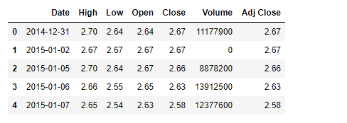

Next, some technical indicators were obtained for the data using the alpha_vantage python package.

接下来，使用alpha_vantage python软件包为数据获取了一些技术指标。

# How to obtain technical indicators for a stock of choice# RSIt_rsi = TechIndicators(key='0E66O7ZP6W7A1LC9',output_format='pandas')data_rsi, meta_data_rsi = t_rsi.get_rsi(symbol='AMD', interval='daily',time_period = 9,                          series_type='open')# Bollinger bandst_bbands = TechIndicators(key='0E66O7ZP6W7A1LC9',output_format='pandas')data_bbands, meta_data_bb = t_bbands.get_bbands(symbol='AMD', interval='daily', series_type='open', time_period=9)

This can easily be functionalized depending on the task. To learn more about technical indicators and how they are useful in stock analysis, I welcome you to explore investopedia’s articles on different technical indicators. Differential data was also included in the list of features for predicting stock prices. In this study, differential data refers to the difference between price information on 2 consecutive days (price at time t and price at time t-1).

可以根据任务轻松地对其进行功能化。 要了解有关技术指标的更多信息，以及它们如何在库存分析中发挥作用 ，我欢迎您浏览investopedia关于不同技术指标的文章。 差异数据也包含在用于预测股价的功能列表中。 在这项研究中，差异数据是指连续2天的价格信息之间的差异(时间t的价格和时间t-1的价格)。

特征工程 (Feature engineering)

Let’s visualize how the generated features relate to each other using a heatmap of the correlation matrix.

让我们使用相关矩阵的热图可视化生成的特征如何相互关联。

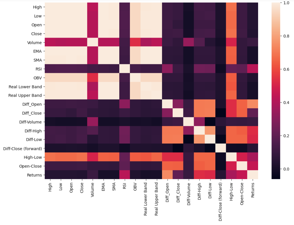
The closing price has very strong correlations with some of the other price information such as opening price, highs, and lows. On the other hand, the differential prices aren't as correlated. We want to limit the amount of colinearity in our system before running any machine learning routine. So feature selection is a must.

收盘价与其他一些价格信息(例如开盘价，最高价和最低价)具有非常强的相关性。 另一方面，差异价格却不相关。 我们希望在运行任何机器学习例程之前限制系统中的共线性量。 因此，功能选择是必须的。

I utilize two means of feature selection in this section. Random forests and mutual information gain. Random forests are very popular due to their relatively good accuracy, robustness as well as simplicity in terms of utilization. They can directly measure the impact of each feature on the accuracy of the model and in essence, give them a rank. Information gain, on the other hand, calculates the reduction in entropy from transforming a dataset in some way. Mutual information gain essentially evaluates the gain of each variable in the context of the target variable.

在本节中，我采用两种功能选择方式。 随机森林和相互信息获取。 随机森林由于其相对较高的准确性，鲁棒性和使用简单性而非常受欢迎。 他们可以直接测量每个功能对模型准确性的影响，并从本质上给他们一个排名。 另一方面，信息增益通过某种方式转换数据集来计算熵的减少。 互信息增益本质上是在目标变量的上下文中评估每个变量的增益。

随机森林回归 (Random forest regressor)

Let’s make a temporary training and testing data sets and run the regressor on it.

让我们做一个临时的训练和测试数据集，并在其上运行回归器。

# Feature selection using a Random forest regressorX_train, X_test,y_train, y_test = train_test_split(X,y,test_size=0.2,random_state=0)feat = SelectFromModel(RandomForestRegressor(n_estimators=100,random_state=0,n_jobs=-1))feat.fit(X_train,y_train)X_train.columns[feat.get_support()]

The regressor essentially selected the features that displayed a good correlation with the close price which is the target variable. However, although it selected the most important we would like information on the information gain from each variable. An issue with using random forests is it tends to diminish the importance of other correlated variables and may lead to incorrect interpretation. However, it does help reduce overfitting. Using the regressor, only three features were seen as being useful for prediction; High, Low, and Open prices.

回归器实质上选择了与作为目标变量的收盘价显示出良好相关性的特征。 但是，尽管它选择了最重要的信息，我们还是希望获得有关每个变量的信息增益的信息。 使用随机森林的一个问题是，它往往会降低其他相关变量的重要性，并可能导致错误的解释。 但是，它确实有助于减少过度拟合。 使用回归器，只有三个特征被认为对预测有用。 高，低和开盘价。

相互信息获取 (Mutual information gain)

Now quantitatively see how each feature contributes to the prediction

现在定量了解每个特征如何有助于预测

from sklearn.feature_selection import mutual_info_regression, SelectKBestmi = mutual_info_regression(X_train,y_train)mi = pd.Series(mi)mi.index = X_train.columnsmi.sort_values(ascending=False,inplace=True)mi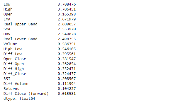

The results validate the results using the random forest regressor, but it appears some of the other variables also contribute a decent amount of information. In terms of selection, only features with contributions greater than 2 are selected, resulting in 8 features

结果使用随机森林回归器验证了结果，但似乎其他一些变量也提供了可观的信息量。 在选择方面，仅会选择贡献大于2的特征，从而产生8个特征

LSTM的数据准备 (Data preparation for the LSTM)

In order to construct a Long short term memory neural network (LSTM), we need to understand its structure. Below is the design of a typical LSTM unit.

为了构建长期短期记忆神经网络(LSTM)，我们需要了解其结构。 以下是典型LSTM单元的设计。

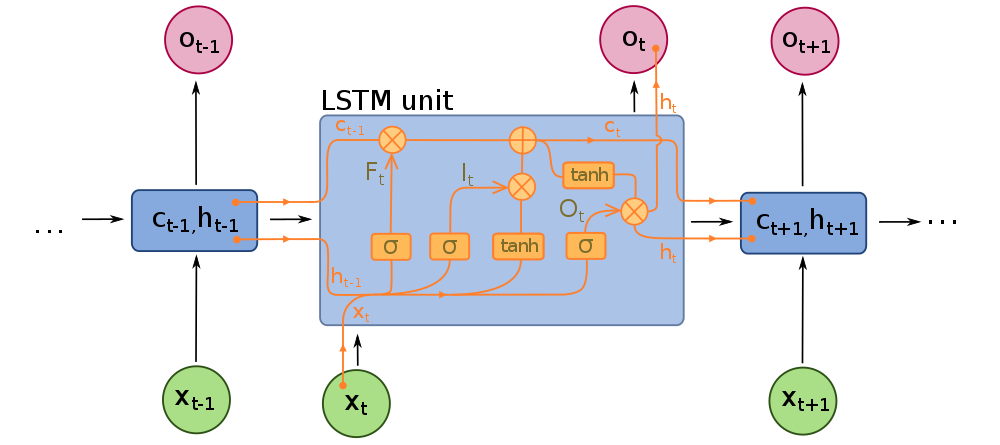
As mentioned earlier, LSTM’s are a special type of recurrent neural network (RNN). Recurrent neural networks (RNN) are a special type of neural network in which the output of a layer is fed back to the input layer multiple times in order to learn from the past data. Basically, the neural network is trying to learn data that follows a sequence. However, since the RNNs utilize past data, they can become computationally expensive due to storing large amounts of data in memory. The LSTM mitigates this issue, using gates. It has a cell state, and 3 gates; forget, input and output gates.

如前所述， LSTM是一种特殊的递归神经网络( RNN )。 递归神经网络( RNN )是一种特殊的神经网络，其中层的输出多次反馈到输入层，以便从过去的数据中学习。 基本上，神经网络正在尝试学习遵循序列的数据。 但是，由于RNN利用过去的数据，由于在内存中存储大量数据，它们可能会在计算上变得昂贵。 LSTM使用盖茨缓解了此问题。 它具有单元状态和3个门。 忘记 ， 输入和输出门。

The cell state is essentially the memory of the network. It carries information throughout the data sequence processing. Information is added or removed from this cell state using gates. Information from the previous hidden state and current input are combined and passed through a sigmoid function at the forget gate. The sigmoid function determines which data to keep or forget. The transformed values are then multiplied by the current cell state.

单元状态本质上是网络的内存。 它在整个数据序列处理过程中都承载信息。 使用门从该单元状态添加或删除信息。 来自先前隐藏状态和当前输入的信息将组合在一起，并通过遗忘门处的S型函数传递。 乙状结肠功能决定要保留或忘记哪些数据。 然后将转换后的值乘以当前单元格状态 。

Next, the information from the previous hidden state (H_(t-1))combined with the input (X_t) is passed through a sigmoid function at the input gate to again determine important information, and also a tanh function to transform data between -1 and 1. This transformation helps with the stability of the network and helps deal with the vanishing/exploding gradient problem. These 2 outputs are multiplied together, and the output is added to the current cell state with the sigmoid function applied to it to give us our new cell state for the next time step.

接下来，来自先前隐藏状态( H_(t-1) )的信息与输入( X_t )的组合将通过输入门的S型函数再次确定重要信息，以及通过tanh函数在-之间转换数据1和1。此转换有助于网络的稳定性，并有助于解决消失/爆炸梯度问题。 将这两个输出相乘，然后将输出加到当前单元格状态，并应用sigmoid函数，为下一步提供新的单元格状态。

Finally, the information from the hidden state combined with the current input is combined and a sigmoid function applied to it. In addition, the new cell state is passed through a tanh function to transform the values and both outputs are multiplied to determine the new hidden state for the next time step at the output gate.

最后，将来自隐藏状态的信息与当前输入组合在一起，并对其应用S型函数。 此外，新的小区状态是通过双曲正切函数传递给变换值和两个输出相乘以确定用于在输出门在下一时间步骤将新的隐藏状态。

Now we have an idea of how the LSTM works, let’s construct one. First, we split our data into training and test set. An 80 – 20 split was used for the training and test sets respectively in this case. The data were then scaled using a MinMaxScaler.

现在我们有了LSTM的工作原理，让我们构造一个。 首先，我们将数据分为训练和测试集。 在这种情况下，分别将80 – 20的比例用于训练和测试集。 然后使用MinMaxScaler缩放数据。

LSTM的数据输入结构 (Structure of data input for LSTM)

The figure below shows how the sequential data for an LSTM is constructed to be fed into the network. Data source: Althelaya et al, 2018

下图显示了如何构造LSTM的顺序数据以馈入网络。 数据来源： Althelaya等人，2018

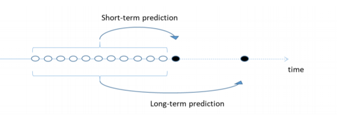
The idea is since stock data is sequential, information on a given day is related to information from previous days. Basically for data at time t, with a window size of N, the target feature will be the data point at time t, and the feature will be the data points [t-1, t-N]. We then sequentially move forward in time using this approach. This applies for the short-term prediction. For long term prediction, the target feature will be Fk time steps away from the end of the window where Fk is the number of days ahead we want to predict. We, therefore, need to format our data that way.

这个想法是因为库存数据是连续的，所以给定日期的信息与前几天的信息有关。 基本上对于时间t的数据，窗口大小为N ，目标特征将是时间t的数据点，特征将是数据点[ t-1 ， tN ]。 然后，我们使用此方法按时间顺序向前移动。 这适用于短期预测。 对于长期预测，目标特征将是距窗口末端的Fk时间步长，其中Fk是我们要预测的提前天数。 因此，我们需要以这种方式格式化数据。

# Formatting input data for LSTMdef format_dataset(X, y, time_steps=1):    Xs, ys = [], []    for i in range(len(X) - time_steps):        v = X.iloc[i:(i + time_steps)].values        Xs.append(v)                ys.append(y.iloc[i + time_steps])    return np.array(Xs), np.array(ys)

Following the work of Althelaya et al, 2018, a time window of 10 days was used for N.

继Althelaya等人(2018年)的工作之后， N使用了10天的时间窗口。

建立LSTM模型 (Building the LSTM model)

The new installment of TensorFlow (Tensorflow 2.0) via Keras has made the implementation of deep learning models much easier than in previous installments. We will apply a bidirectional LSTM as they have been shown to more effective in certain applications (see Althelaya et al, 2018). This due to the fact that the network learns using both past and future data in 2 layers. Each layer performs the operations using reversed time steps to each other. The loss function, in this case, will be the mean squared error, and the adam optimizer with the default learning rate is applied. 20% of the training set will also be used as a validation set while running the model.

通过Keras的TensorFlow新版(Tensorflow 2.0)使深度学习模型的实现比以前的版本容易得多。 我们将应用双向LSTM，因为它们已被证明在某些应用中更有效(请参见Althelaya等人，2018年 )。 这是由于网络在2层中同时使用过去和将来的数据进行学习。 每一层使用彼此相反的时间步长执行操作。 在这种情况下，损失函数将是均方误差，并且将使用具有默认学习率的adam优化器。 运行模型时，训练集的20％也将用作验证集。

# Design and input arguments into the LSTM model for stock price predictionfrom tensorflow import keras# Build model. Include 20% drop out to minimize overfittingmodel = keras.Sequential()model.add(keras.layers.Bidirectional(        keras.layers.LSTM(          units=32,           input_shape=(X_train_lstm.shape[1], X_train_lstm.shape[2]))  ))model.add(keras.layers.Dropout(rate=0.2))model.add(keras.layers.Dense(units=1))# Define optimizer and metric for loss functionmodel.compile(optimizer='adam',loss='mean_squared_error')# Run modelhistory = model.fit(    X_train_lstm, y_train_lstm,     epochs=90,     batch_size=40,     validation_split=0.2,    shuffle=False,    verbose=1   )

Note we do not shuffle the data in this case. That’s because stock data is sequential i.e the price on a given day is dependent on the price from previous days. Now let’s have a look at the loss function to see how the validation and training data fair

请注意，在这种情况下，我们不会对数据进行混洗。 这是因为库存数据是连续的，即给定日期的价格取决于前几天的价格。 现在让我们看一下损失函数，看看验证和训练数据如何公平

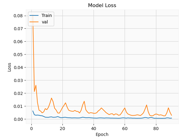
The validation set appears to have a lot more fluctuations relative to the training set. This is mainly due to the fact that most neural networks use stochastic gradient descent in minimizing the loss function which tends to be stochastic in nature. In addition, the data is batched which can influence the behavior of the solution. Of course, ideally, these hyper-parameters need to be optimized, but this is merely a simple demonstration. Let’s have a look at the solution

相对于训练集，验证集似乎有更多的波动。 这主要是由于以下事实：大多数神经网络使用随机梯度下降来使损失函数最小化，而损失函数在本质上往往是随机的。 此外，数据会被批处理，这可能会影响解决方案的行为。 当然，理想情况下，需要优化这些超参数，但这仅仅是一个简单的演示。 让我们看一下解决方案

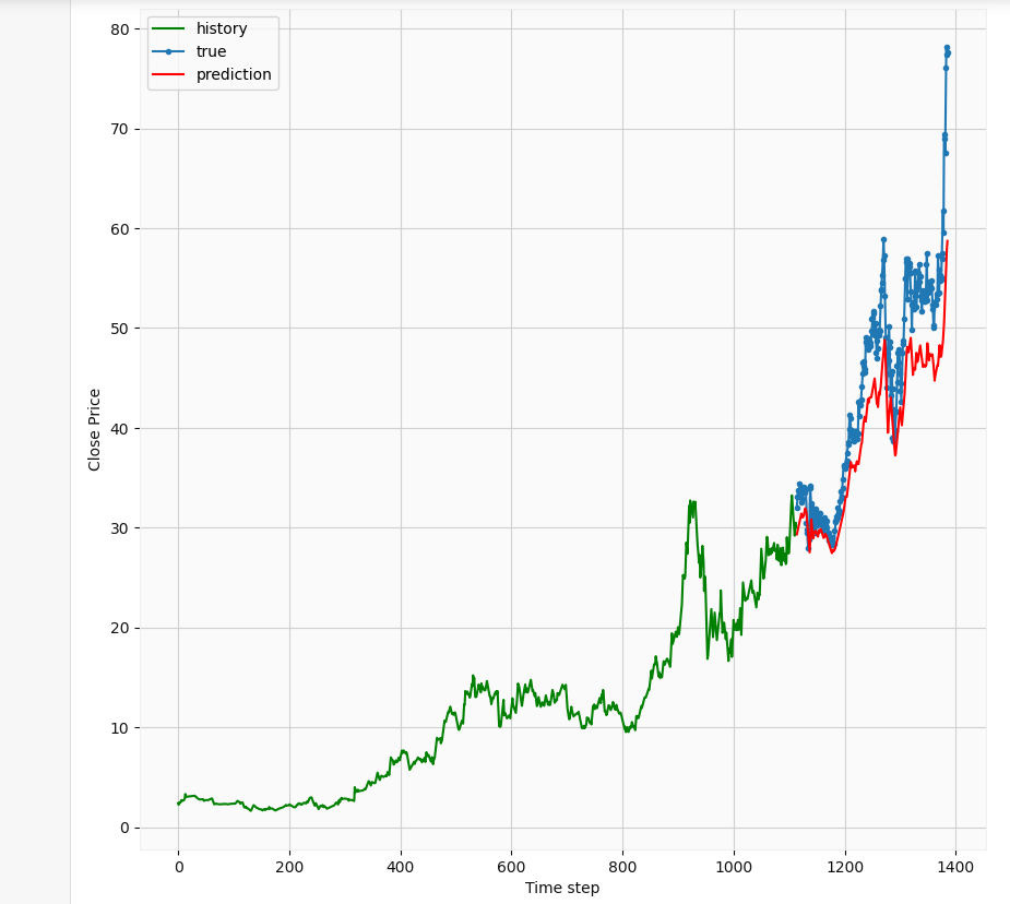
Overall, it seems the predictions follow the trend of the actual prices. Of course with more epochs and hyperparameter tuning, we could achieve better results. Let’s take a closer look

总体而言，似乎这些预测遵循实际价格的趋势。 当然，通过更多的时期和超参数调整，我们可以获得更好的结果。 让我们仔细看看

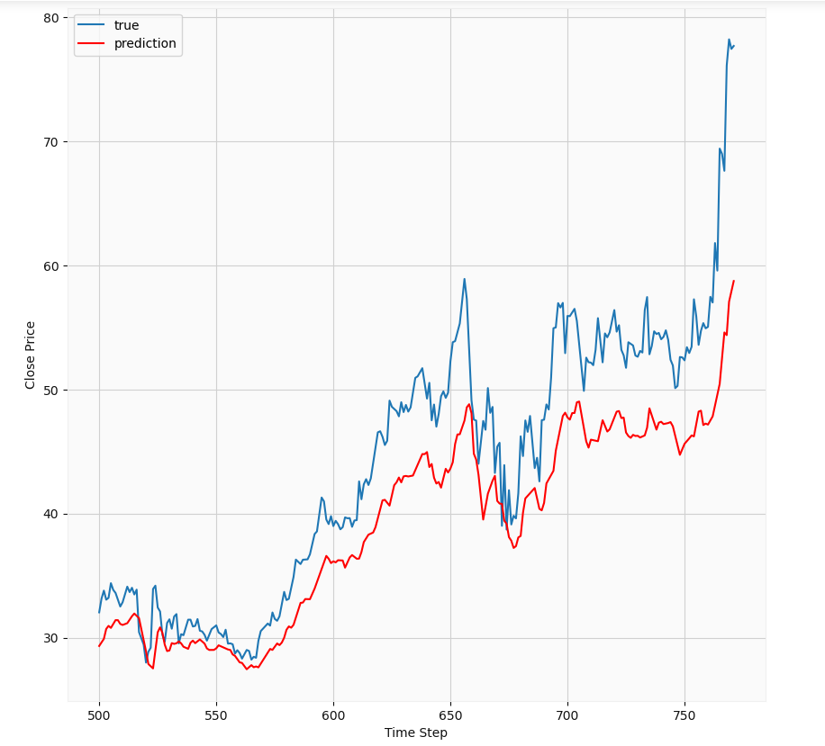
At first glance, we notice the LSTM has some implicit autocorrelation in its results since its predictions for a given day are very similar to those of the previous day. The predictions essentially lag the true results. Its basically showing that the best guess of the model is very similar to previous results. This should not be a surprising result; The stock market is influenced by a number of factors such as news, earnings reports, mergers, etc. Therefore, it is a bit too chaotic and stochastic to be accurately modeled because it depends on so many factors, some of which can be sporadic i.e positive or negative news. Therefore, in my opinion, this may not be the best way to predict stock prices. Of course with major advances in AI, there might actually be a way of doing this using LSTMs, but I don’t think the hedge funds will be sharing their methods with outsiders anytime soon.

乍一看，我们注意到LSTM在其结果中具有一些隐式自相关，因为它在给定日期的预测与前一天的预测非常相似。 这些预测实质上落后于真实结果。 它基本上表明，模型的最佳猜测与以前的结果非常相似。 这应该不足为奇； 股票市场受到许多因素的影响，例如新闻，收益报告，合并等。因此，它过于混乱和随机，无法准确建模，因为它取决于太多因素，其中一些因素可能是零星的，即正面或负面新闻。 因此，我认为，这可能不是预测股价的最佳方法。 当然，随着AI的重大进步，实际上可能有一种使用LSTM做到这一点的方法，但是我认为对冲基金不会很快与外界共享其方法。

第3部分：使用回归分析估算价格走势 (Part 3: Estimating price movement with regression analysis)

Of course, we could still make an attempt to have an idea of what the possible price movements might be. In this case, I will utilize the differential prices as there is less variance compared to using absolute prices. This is a somewhat naive way but let’s try it nevertheless. Let’s explore some relationships

当然，我们仍然可以尝试了解价格可能发生的变化。 在这种情况下，我将利用差异价格，因为与使用绝对价格相比，差异较小。 这是一种比较幼稚的方法，但是还是请尝试一下。 让我们探索一些关系

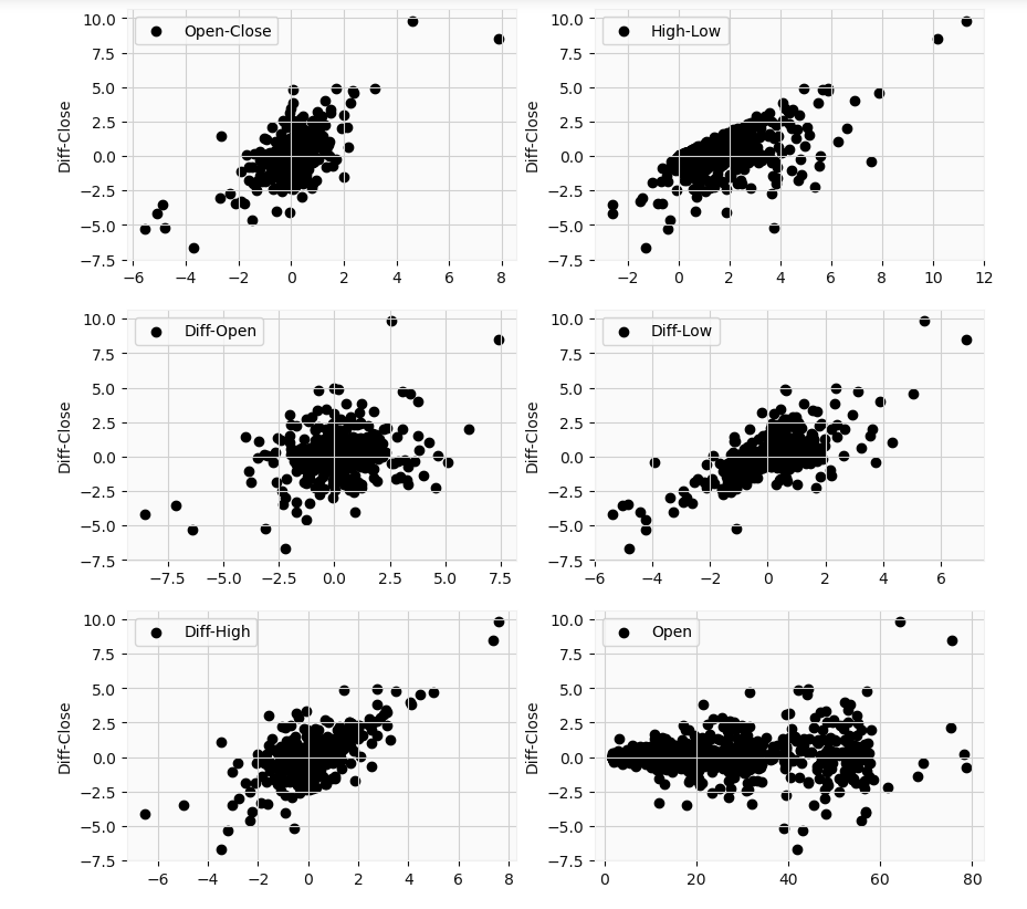
Again to reiterate, the differential prices relate to the difference between the price at time t and the previous day value at time t-1. The differential high, differential low, differential high-low, and differential open-close price appear to have a linear relationship with the differential close. But only the differential open-close would be useful in analysis. This because on a given day (time t), we can not know what the highs or lows are beforehand till the end of the trading day. Theoretically, those values could end up coinciding with the closing price. However, we do know the open value at the start of the trading period. I will apply ridge regression to make our results more robust. Our target variable will be the differential close price, and our feature will be the differential open-close price.

再次重申，差异价格与时间t的价格和时间t-1的前一天值之间的差有关。 差价高，差价低，差价高低和差价开盘价与差价收盘价似乎具有线性关系。 但是，只有微分开闭对分析有用。 这是因为在给定的一天(时间t )，我们直到交易日结束之前都不知道高点或低点是什么。 从理论上讲，这些价值最终可能与收盘价一致。 但是，我们确实知道交易期开始时的未平仓价。 我将应用岭回归来使我们的结果更可靠。 我们的目标变量将是差异收盘价，而我们的特征将是差异开盘价。

from sklearn.linear_model import LinearRegression, Ridge, Lassofrom sklearn.model_selection import GridSearchCV, cross_val_scoreimport sklearnfrom sklearn.metrics import median_absolute_error, mean_squared_error# Split data into training and testX_train_reg, X_test_reg, y_train_reg, y_test_reg = train_test_split(X_reg, y_reg, test_size=0.2, random_state=0)# Use a 10-fold cross validation to determine optimal parameters for a ridge regressionridge = Ridge()alphas = [1e-15,1e-8,1e-6,1e-5,1e-4,1e-3,1e-2,1e-1,0,1,5,10,20,30,40,45,50,55,100]params = {'alpha': alphas}ridge_regressor = GridSearchCV(ridge,params, scoring='neg_mean_squared_error',cv=10)ridge_regressor.fit(X_reg,y_reg)print(ridge_regressor.best_score_)print(ridge_regressor.best_params_)

The neg_mean_squared_error returns the negative version of the mean squared error. The closer it is to 0, the better the model. The cross-validation returned an alpha value of 1e-15 and a score of approximately -0.4979. Now let’s run the actual model and see our results

neg_mean_squared_error返回均方误差的负版本。 距离0越近，模型越好。 交叉验证返回的alpha值为1e-15，得分约为-0.4979。 现在让我们运行实际模型并查看我们的结果

regr = Ridge(alpha=1e-15)regr.fit(X_train_reg, y_train_reg)y_pred = regr.predict(X_test_reg)y_pred_train = regr.predict(X_train_reg)print(f'R^2 value for test set is {regr.score(X_test_reg,y_test_reg)}')print(f'Mean squared error is {mean_squared_error(y_test_reg,y_pred)}')plt.scatter(df_updated['Open-Close'][1:],df_updated['Diff_Close'][1:],c='k')plt.plot(df_updated['Open-Close'][1:], (regr.coef_[0] * df_updated['Open-Close'][1:] + regr.intercept_), c='r' );plt.xlabel('Open-Close')plt.ylabel('Diff-Close')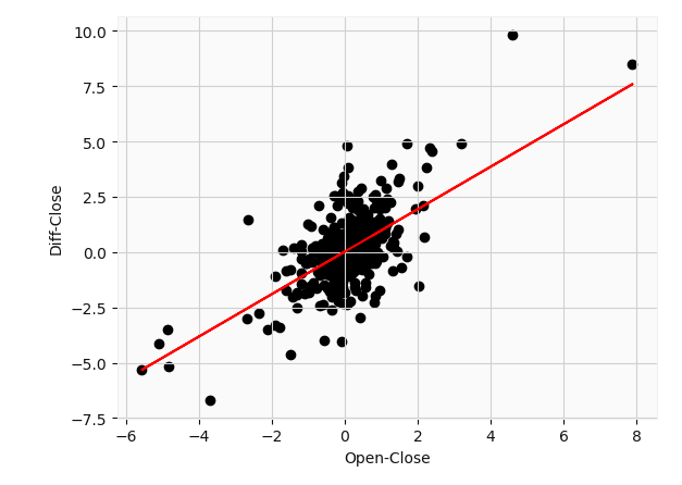

The model corresponds to a slope of $0.9599 and an intercept of $0.01854. This basically says that for every $1 increase in price between the opening price on a given day, and its previous closing price we can expect the closing price to increase by roughly a dollar from its closing price the day before. I obtained a mean square error of 0.58 which is fairly moderate all things considered. This R² value of 0.54 basically says 54% of the variance in the differential close price is explained by the differential open-close price. Not so bad so far. Note that the adjusted R² value was roughly equal to the original value.

该模型对应的斜率是0.9599美元 ，截距是0.01854美元。 这基本上就是说，在给定日期的开盘价与其之前的收盘价之间，每增加1美元的价格，我们就可以预期收盘价比前一天的收盘价增加大约1美元。 我获得了0.58的均方误差，考虑到所有因素，该误差相当适中。 R2值为0.54基本上表示差异收盘价差异的54％由差异开盘价解释。 到目前为止还算不错。 请注意，调整后的R²值大致等于原始值。

To be truly effective, we need to make further use of statistics. Specifically, let’s define a prediction interval around the model. Prediction intervals give you a range for the prediction that accounts for any threshold of modeling error. Prediction intervals are most commonly used when making predictions or forecasts with a regression model, where a quantity is being predicted. We select the 99% confidence interval in this example such that our actual predictions fall into this range 99% of the time. For an in-depth overview and explanation please explore machinelearningmastery

为了真正有效，我们需要进一步利用统计数据。 具体来说，让我们在模型周围定义一个预测间隔。 预测间隔为您提供了一个预测范围，该范围考虑了建模误差的任何阈值。 预测间隔是在预测数量的回归模型中进行预测或预测时最常使用的时间间隔。 在此示例中，我们选择99％置信区间，以使我们的实际预测有99％的时间处于该范围内。 有关深入的概述和说明，请浏览机器学习知识。

def predict_range(X,y,model,conf=2.58):

    from numpy import sum as arraysum

    # Obtain predictions    yhat = model.predict(X)

    # Compute standard deviation    sum_errs = arraysum((y - yhat)**2)    stdev = np.sqrt(1/(len(y)-2) * sum_errs)

    # Prediction interval (default confidence: 99%)    interval = conf * stdev

    lower = []    upper = []

    for i in yhat:        lower.append(i-interval)        upper.append(i+interval)return lower, upper, interval

Let’s see our prediction intervals

让我们看看我们的预测间隔

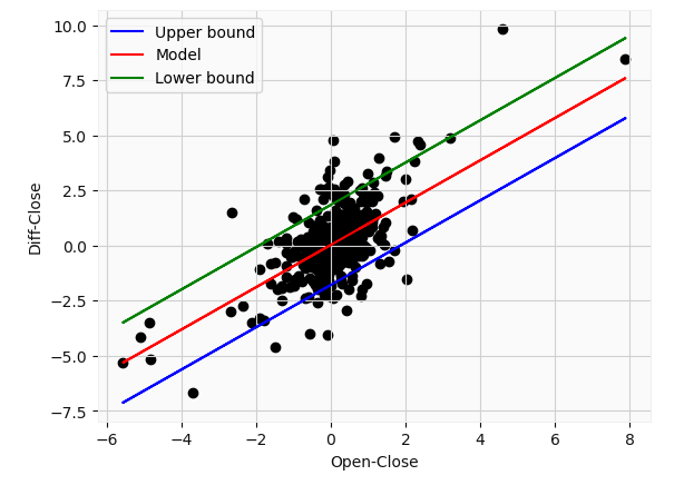
Our prediction error corresponds to a value of $1.82 in this example. Of course, the parameters used to obtain our regression model (slope and intercept) also have a confidence interval which we could calculate, but its the same process as highlighted above. From this plot, we can see that even with a 99% confidence interval, some values still fall outside the range. This highlights just how difficult it is to forecast stock price movements. So ideally we would supplement our analysis with news, technical indicators, and other parameters. In addition, our model is still quite limited. We can only make predictions about the closing price on the same day i.e at time t. Even with the large uncertainty, this could potentially prove useful in, for instance, options tradings.

在此示例中，我们的预测误差对应于$ 1.82的值。 当然，用于获得回归模型的参数(斜率和截距)也具有我们可以计算的置信区间，但其过程与上面突出显示的过程相同。 从该图可以看出，即使置信区间为99％，某些值仍落在该范围之外。 这突显了预测股价走势的难度。 因此，理想情况下，我们将使用新闻，技术指标和其他参数来补充我们的分析。 此外，我们的模型仍然非常有限。 我们只能对当天(即时间t)的收盘价做出预测。 即使存在很大的不确定性，这也可能在例如期权交易中被证明是有用的。

这是什么意思呢？ (What does this all mean?)

The stock screening strategy introduced could be a valuable tool for finding good stocks and minimizing loss. Certainly, in future projects, I could perform sentiment analysis myself in order to get information on every stock from the biggest movers list. There is also some room for improvement in the LSTM algorithm. If there was a way to minimize the bias and eliminate the implicit autocorrelation in the results, I’d love to hear about it. So far, the majority of research on the topic haven’t shown how to bypass this issue. Of course, more model tuning and data may help so any experts out there, please give me some feedback. The regression analysis seems pretty basic but could be a good way of adding extra information in our trading decisions. Of course, we could have gone with a more sophisticated approach; the differential prices almost appear to form an ellipse around the origin. Using a radial SVM classifier could also be a potential way of estimating stock movements.

引入的库存筛选策略可能是寻找优质库存并最大程度减少损失的有价值的工具。 当然，在未来的项目中，我可以自己进行情绪分析，以便从最大的推动者名单中获取每只股票的信息。 LSTM算法还有一些改进的余地。 如果有一种方法可以最大程度地减少偏差并消除结果中隐式的自相关，我很想听听它。 到目前为止，有关该主题的大多数研究都没有显示如何绕过此问题。 当然，更多的模型调整和数据可能会有所帮助，所以那里的任何专家都请给我一些反馈。 回归分析似乎很基础，但可能是在我们的交易决策中添加额外信息的好方法。 当然，我们可以采用更复杂的方法。 差价似乎在原产地周围形成了椭圆形。 使用径向SVM分类器也可能是估计库存运动的一种潜在方法。

The codes, as well as the dataset, will be provided here in the not so distant future, and my Linkedin profile can be found here. Thank you for reading!

在不久的将来会在此处提供代码和数据集，我的Linkedin个人资料可在此处找到。 感谢您的阅读！

Ibinabo Bestmann

伊比纳博·贝斯特曼